- 19.1 Basic Relationships in Fluid Mechanics
- 19.2 Fluid Flow Equipment
- 19.3 Frictional Pipe Flow
- 19.4 Other Flow Situations
- 19.5 Performance of Fluid Flow Equipment
- References
- Short Answer Questions
- Problems
This chapter is from the book
This chapter is from the book
This chapter is from the book
19.5 Performance of Fluid Flow Equipment
In addition to equipment design, the chemical engineer must deal with the performance of existing equipment. The differences between the design problem (also called a rating problem) (a) and the performance problem (b) are illustrated in Figure 19.17. The use of italics indicates the unknowns in the particular problem. In the design problem, the input and the desired output are specified, and the equipment is designed to satisfy those constraints. In the performance problem, the input and equipment are specified, and the output is determined. The performance problem is what is involved in dealing with day-to-day operations in a chemical plant.
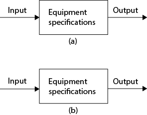
Figure 19.17 Illustrations of (a) Design Problem and (b) Performance Problem (Unknowns Are Indicated by Italics for Each Case)
Several different types of problems in frictional fluid flow using the mechanical energy balance were discussed in Section 19.3. Determining the pump power needed for a given situation is a design problem. Similarly, determining the required pipe diameter is a design problem. On the other hand, determining the flowrate when all equipment is specified is a performance problem, as is determining the pressure change for an existing system.
Suppose it is necessary to increase the capacity of a process without adding new equipment. Logically, all flowrates must increase. This is a performance problem, since the input and equipment are specified, and the output must be determined for each unit in the process. Somewhere in the process, the amount of scale-up needed will be limited due to equipment constraints, and this limiting unit is called a bottleneck. The process of finding a solution that removes the bottleneck is called debottlenecking, which is a performance problem. Similarly, if there is a problem with the output of a process (purity or temperature, for example), the cause of the problem must be determined, which is called troubleshooting.
Returning to the situation in which process capacity must be increased, for the fluid flow component, initially, it may appear that problems similar to those in Section 19.3 must be solved from scratch. However, for many situations, not just in fluid flow, very good approximations can be made with a much simpler analysis.
19.5.1 Base-Case Ratios
The ability to predict changes in a process design or in plant operations is improved by anchoring an analysis to a base case. This calculation tool combines use of fundamental relationships with plant operating data to form a basis for predicting changes in system behavior. As will be seen, it is applicable to problems involving all chemical process units when analytical expressions are available.
For design changes, it is desirable to identify a design proven in practice as the base case. For operating plants, actual data are available and are chosen as the base case. It is important to put this base case into perspective. Assuming that there are no instrument malfunctions and these operating data are correct, then these data represent a real operating point at the time the data were taken. As the plant ages, the effectiveness of process units changes and operations are altered to account for these changes. As a consequence, recent data on plant operations should be used in setting up the base case.
The base-case ratio integrates the “best available” information from the operating plant with design relationships to predict the effect of process changes. It is an important and powerful technique with a wide range of applications. The base-case ratio, X, is defined as the ratio of a new-case system characteristic, x2, to the base-case system characteristic, x1:
)
Using a base-case ratio often reduces the need for knowing actual values of physical properties (physical properties refer to thermodynamic and transport properties of fluids), equipment, and equipment characteristics. The values identified in the ratios fall into three major groups. They are defined below and applied in Examples 19.15 and 19.16.
Ratios Related to Equipment Sizes (equivalent length, Leq; diameter, D; surface area, A): Assuming that the equipment is not modified, these values are constant, the ratios are unity, and these terms cancel out.
Ratios Related to Physical Properties (such as density, ρ; viscosity, μ): These values can be functions of material composition, temperature, and pressure. Only the functional relationships, not absolute values, are needed. For small changes in composition, temperature, or pressure, the properties often are unchanged, and the ratio is unity and cancels out. An exception to this is gas-phase density.
Ratios Related to Stream Properties: These ratios usually involve velocity, flowrate, concentration, temperature, and pressure.
Using the base-case ratio eliminates the need to know equipment characteristics and reduces the amount of physical property data needed to predict changes in operating systems.
The base-case ratio is a powerful and straightforward tool to analyze and predict process changes. This is illustrated in Example 19.15.
Example 19.15
It is necessary to scale up production in an existing chemical plant by 25%. Your job is to determine whether a particular pump has sufficient capacity to handle the scale-up. The pump’s function is to provide enough pressure to overcome frictional losses between the pump and a reactor.
Solution
The relationship for frictional pressure drop is obtained from the mechanical energy balance:
)
This relationship is now written as the ratio of two cases, where subscript 1 indicates the base case, and subscript 2 indicates the new case:
)
Because the pipe has not been changed, the ratios of diameters (D2/D1) and lengths (Leq2/Leq1) are unity. Because a pump is used only for liquids, and liquids are (practically) incompressible, the ratio of densities is unity. If the flow is assumed to be fully turbulent, which is usually true for process applications, the friction factor is not a function of Reynolds number. This fact should be checked for a particular application. Figure 19.6 illustrates how, for fully turbulent flow in pipes that are not hydraulically smooth, the friction factor approaches a constant value. Since the x-axis is a log scale, changes up to a factor of 2 to 5, which are well beyond the scale-up capability of most equipment, do not represent much of a difference on the graph. Therefore, the friction factor is constant, and the ratio of friction factors is unity. The ratio in Equation (E19.15b) reduces to
)
where the second equality is obtained by substituting for ui in numerator and denominator using the mass balance  , canceling the ratio of densities for the same reason as above, and canceling the ratio of cross-sectional areas because the pipe has remained unchanged. Therefore, by assigning the base-case mass flow to have a value of 1, for a 25% scale-up, the new case has a mass flow of 1.25, and the ratio of pressure drops becomes
)
Thus, the pump must be able to deliver enough head to overcome 56% additional frictional pressure drop while pumping 25% more material.
It is important to observe that Example 19.15 was solved without knowing any details of the system. The pipe diameter, length, and number of valves and fittings were not known. The liquid being pumped, its temperature, and its density were not known. Yet the use of base-case ratios along with simple assumptions permitted a solution to be obtained. This illustrates the power and simplicity of base-case ratios.
Example 19.16
It is proposed to improve performance through a section of pipe by adding an identical section in parallel.
If the total flowrate remains constant, what parameter changes and by how much, assuming the fluid flow is fully turbulent?
If the original pipe is 1.5-in, schedule-40, commercial steel, and the new section is 2-in, schedule-40, commercial steel, answer the same question as in Part (a).
Solution
By using the mechanical energy balance and Equation (19.14) for the friction term, with the subscript 1 representing the original case and subscript 2 representing the new case, each being the flow through the original section, the ratio of pressure drops is
The constants cancel. If the fluid is unchanged, the densities cancel. Since the new and old pipe lengths and diameters are identical, the lengths and diameters cancel. It is assumed that the minor losses due to the elbows and fitting needed to add the parallel pipe are unchanged, so the equivalent lengths cancel. For fully turbulent flow, the friction factor has asymptotically approached a constant value (Figure 19.6), so the friction factors cancel. So, the result is
Since the two parallel sections are identical, the flowrate splits equally between the two sections, so the flowrate in the original section is half of the original flowrate:
Therefore, the pressure drop through that section of pipe decreases by 75%.
In this case, subscripts 1 and 2 represent the flow though the original and new sections, after the parallel section is installed. The analysis starts identically, but the diameters and friction factors do not cancel. The friction factors do not cancel because the asymptotic value for the friction factor in Figure 19.6 and in the Pavlov equation (Equation [19.16]) depends on the ratio of the roughness factor to the diameter, and that ratio is different for the two sections of pipe. The ratio expression becomes
From the Pavlov equation (Equation [19.16]), using the ratio of the friction factors at an asymptotically large Reynolds number and the schedule pipe diameters, Equation (E19.16d) becomes
Since the pressure drops in each parallel section must be equal,
If the flow is laminar, the analysis would be similar, but the results would differ due to the different expression for the friction factor in laminar flow. Examples of this are the subject of problems at the end of the chapter.
)
)
)
)
)
)
19.5.2 Net Positive Suction Head
There is a significant limitation on pump operation called net positive suction head (NPSH). This is the head that is needed on the pump feed (suction) side to ensure that liquid does not vaporize upon entering the pump. Its origin is as follows. Although the effect of a pump is to raise the pressure of a liquid, frictional losses at the entrance to the pump, between the suction pipe and the internal pump mechanism, cause the liquid pressure to drop upon entering the pump. This means that a minimum pressure exists somewhere within the pump. If the feed liquid is saturated or nearly saturated, the liquid can vaporize upon entering due to this internal pressure drop. This causes formation of vapor bubbles. These bubbles rapidly collapse when exposed to the forces created by the pump mechanism, called cavitation. This process usually results in noisy pump operation and, if it occurs for a period of time, will damage the pump. As a consequence, regulating valves, which lower fluid pressure, are not normally placed in the suction line to a pump.
Pump manufacturers supply NPSH data with a pump, usually in head units. In this book, both head and pressure units are used. The required NPSH, denoted NPSHR, is a function of the square of velocity because it is a frictional loss and because most applications involve turbulent flow. Figure 19.18(a) shows NPSHR and NPSHA curves, which define a region of acceptable pump operation. This is specific to a given liquid. Typical NPSHR values are in the range of 15 to 30 kPa (2-4 psi) for small pumps and can reach 150 kPa (22 psi) for larger pumps. Figure 19.18 also shows curves for NPSHA, the available NPSH, along with the NPSHR curve.
)
Figure 19.18 (a) NPSHA and NPSHR Curves Showing Region of Feasible Operation; (b) How Physical Parameters Affect Shape of NPSHA Curve
The available NPSHA is defined as
)
Equation (19.66) means that the available NPSH (NPSHA) is the difference between the inlet pressure, Pinlet, and P*, which is the vapor pressure (bubble-point pressure for a mixture). It is required that NPSHA ≥ NPSHR to avoid cavitation. Cavitation is avoided if operation is to the left of the intersection of the two curves. It is physically possible to operate to the right of the intersection of the two curves, but doing so is not recommended because the pump will be damaged.
All that remains is to calculate or know the pump inlet conditions in order to determine whether sufficient NPSH (NPSHA) is available to equal or exceed the required NPSH (NPSHR). For example, consider the exit stream from a distillation column reboiler, which is saturated liquid. If it is necessary to pump this liquid, cavitation could be a problem. A common solution to this problem is to elevate the column above the pump so that the static pressure increase minus any frictional losses between the column and the pump provides the necessary NPSH to avoid cavitation. This can be done either by elevating the column above ground level using a metal skirt or by placing the pump in a pit below ground level, although pump pits are usually avoided due to safety concerns arising from accumulation of heavier-than-air gases in the pit.
In order to quantify NPSH, consider Figure 19.19, in which material in a storage tank is pumped downstream in a chemical process. This scenario is a very common application of the NPSH concept. For NPSH analysis, the only portion of Figure 19.19 under consideration is between the tank and pump inlet.
)
Figure 19.19 Typical Situation for Application of NPSH Principles
From the mechanical energy balance, the pressure at the pump inlet can be calculated to be
)
which means that the pump inlet pressure is the tank pressure plus the static pressure minus the frictional losses in the suction-side piping. Therefore, by substituting Equation (19.67) into Equation (19.66), the resulting expression for NPSHA is
)
This is an equation of a concave downward parabola, of the form 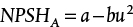 , as illustrated in Figure 19.18(b), Curve a. The intercept is a = Ptank + pgh − P* and b = 2ρfLeq/D. This analysis does not include the kinetic energy term due to the acceleration of the fluid from the tank into the pipe. Rigorously, this term should also be included in the analysis.
If NPSHA is insufficient for a particular situation, Equation (19.68) suggests methods to increase the NPSHA:
Decrease the temperature of the liquid at the pump inlet. This decreases the value of the vapor pressure, P*, thereby increasing NPSHA. This increases the intercept of the NPSHA curve while maintaining constant curvature, as illustrated in Figure 19.18(b), Curve b.
Increase the static head. This is accomplished by increasing the value of h in Equation (19.64), thereby increasing NPSHA. As was said earlier, pumps are most often found at lower elevations than the source of the material they are pumping. This increases the intercept of the NPSHA curve while maintaining constant curvature, as illustrated in Figure 19.18(b), Curve b.
Increase the tank pressure. This increases the intercept of the NPSHA curve while maintaining constant curvature, as illustrated in Figure 19.18(b), Curve b.
Increase the diameter of the suction line (feed pipe to pump). This reduces the velocity and the frictional loss term, thereby increasing NPSHA. This decreases the curvature of the NPSHA curve, as illustrated in Figure 19.18(b), Curve c. It is standard practice to have larger-diameter pipes on the suction side of a pump than on the discharge side.
Example 19.17 illustrates how to do NPSH calculations and one of the preceding methods for increasing NPSHA. The other methods are illustrated in problems at the end of the chapter.
Example 19.17
A pump is used to transport toluene at 10,000 kg/h from a feed tank (V-101) maintained at atmospheric pressure and 57°C. The pump is located 2 m below the liquid level in the tank, and there is 6 m of equivalent pipe length between the tank and the pump. It has been suggested that 1-in, schedule-40, commercial-steel pipe be used for the suction line. Determine whether this is a suitable choice. If not, suggest methods to avoid pump cavitation.
Solution
The following data can be found for toluene: ln P*(bar) = 10.97 − 4203.06/T(K), μ = 4.1 × 10⁻⁴ kg/m s, ρ = 870 kg/m3. For 1-in, schedule-40, commercial-steel pipe, the roughness factor is about 0.001 and the inside diameter is 0.02664 m. Therefore, the velocity of toluene in the pipe can be found to be 5.73 m/s. The Reynolds number is about 426,000, and the friction factor is f = 0.005. At 57°C, the vapor pressure is found to be 0.172 bar.
From Equation (19.68),
)
This is shown as Point A on Figure 19.18(b). At the calculated velocity, Figure 19.18(b) shows that NPSHR is 0.40 bar, Point B. Therefore, there is insufficient NPSHA. This means that a 1-in, schedule-40 pipe is unacceptable for this service.
The obvious solution to this problem is to use a larger-diameter pipe for the suction side of the pump. The calculated velocity of 5.73 m/s is far in excess of the typical maximum liquid velocity. The frictional loss in the 6 m of suction piping is approximately 0.64 bar. If, say, a 2-in, schedule-40 pipe was used for the suction line, then the frictional loss would decrease to approximately 0.02 bar and NPSHA would increase to about 0.99 bar, which is far in excess of NPSHR. Another method for increasing NPSHA is to increase the height of liquid in the tank. If the height of liquid in the tank is 3 m, with the original 1-in, schedule-40 pipe at the original temperature, NPSHA = 0.445 bar. This is shown as Point C on Figure 19.18(b).
19.5.3 Pump and System Curves
Pumps also have characteristic performance curves, called pump curves. Figure 19.20 illustrates a pump curve for a centrifugal pump. Centrifugal pumps are often called constant head pumps because, over a wide range of volumetric flowrates, the head produced by the pump is approximately constant. Pump manufacturers provide the characteristic curve, usually in head units. For centrifugal pumps, the shape of the curve indicates that although the head remains constant over quite a wide range of flowrates, eventually, as the flowrate continues to increase, the head produced decreases. Pump curves also include power and efficiency curves, both of which change with flowrate and head; however, these are not shown here.
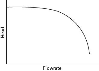
Figure 19.20 Typical Shape of Pump Curve for Centrifugal Pump
For a piping system, a system curve can also be defined. Consider the system as illustrated in Figure 19.21. Location 1 is called the source, and Location 2 is the destination. Location 2 may be distant from Location 1, perhaps at the opposite end of a chemical process and at a different elevation from Location 1. Typical processes have only one pump upstream to supply all pressure needed to overcome pressure losses throughout the process. Therefore, the pressure increase across the pump must be sufficient to overcome all of the losses associated with piping and fittings plus the indicated pressure loss across the control valve. The orifice plate is present to illustrate some type of flowrate measurement, and the flow indicator controller (FIC) illustrates that the measured flowrate is compared to a set point, and deviations from the set point are compensated by adjusting the valve, usually pneumatically. If the flowrate is too large, the valve is partially closed, restricting the flowrate. However, this also increases the frictional pressure loss across the valve, as discussed in Section 19.3.2.
)
Figure 19.21 Physical Situation for System Curve
The behavior of the system can be quantified by a system curve. The general equation for a chemical process, in terms of pressure, is given by the mechanical energy balance between Points 1 and 2 in Figure 19.21:
)
where
)
Equation (19.70) is derived from the mechanical energy balance with only the pressure and friction terms. It is important to remember that Δ represents out-in; therefore, the frictional loss term and the pressure loss across the valve are negative numbers before the included negative sign. The system curve is the right-hand side of Equation (19.69) without the term for the control valve:
)
Equation (19.71) is a parabola, concave upward, on a plot of pressure increase versus flowrate. It is of the form 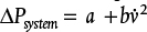 , where a = (P2 − P1) + ρ g(z2 −z1) and
 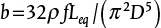 . Since the manufacturer pump curve is usually provided in head units, Equation (19.69) can be rewritten in head units as
)
Figure 19.22 illustrates the result if the pump curve and the system curve are plotted on the same graph. The indicated pressure changes demonstrate how the head provided by the pump must equal the desired head increase from source to destination, plus the frictional pressure loss, plus the pressure loss across the control valve, as quantified in Equation (19.69). The process of flowrate regulation is also illustrated in Figure 19.22. If the flowrate is to be reduced, the valve is closed, and the operating point moves to the left. At this lower flowrate, the frictional losses are lower, but the pressure loss across the valve is larger. The opposite is true for a higher flowrate. At the intersection of the two curves, the valve is wide open, and the maximum possible flowrate has been reached. This analysis assumes that the pump is operating at constant speed. For a variable speed pump, the pump curve moves up or down as the speed of rotation of the impeller changes. (Note that this simplified explanation omits the very small pressure drop across a wide-open control valve.) Operation to the right of this point is impossible. It is important not to confuse the meanings of the intersection points on the pump-system curve plot and the NPSH plot.
)
Figure 19.22 Pump (Constant Speed Centrifugal Pump) and System Curve Components
The pump and system curve plot also illustrates the cost of flowrate regulation. The pump must provide sufficient pressure to overcome the losses across the valve over a wide range of flowrates. Additional pump power is required for the possibility of operating at lower flowrates with a very large pressure drop across the valve. In general, this is a small cost for a pump, because the liquid density is high. Variable speed pumps are also available with different pump curves for different speeds. For these, the flowrate is regulated by the rotation speed of the impeller, not by a valve. It is not usually worth the extra cost for small pumps given the low cost of pumping liquids but may be worth considering for larger pumps and flowrates. Pumps with different impeller sizes have different pump curves for each impeller size. However, changing an impeller is not something that can be done while a process is operating.
Pumps (and compressors) are about the only pieces of equipment in a chemical plant with moving parts. Moving parts can fail. Therefore, since pumps are often inexpensive (on the order of $10,000), a backup pump is typically installed in parallel so the plant can continue operating while the primary pump is maintained. Since shutdown and start-up can take days, it makes sense not to shut down a process that generates profit at a rate of thousands of dollars per minute to avoid purchasing a relatively inexpensive backup pump.
The presence of a backup pump can also be exploited if is necessary to scale-up a process. The piping system can be constructed such that the two pumps can operate simultaneously, either in series or in parallel. If the pumps are in series, the head increase doubles at the same flowrate. If the pumps are in parallel, the flowrate doubles at the same head increase. The pump curves for these situations are illustrated in Figure 19.23. The two system curves illustrate the maximum possible scale-up for two different system curves, indicated by the dots. In one case, the parallel configuration provides more scale-up potential, and in the other case, the series configuration provides more scale-up potential. This demonstrates that it is not possible to make any generalizations about which configuration can produce more scale-up. It all depends on the particular system.
)
Figure 19.23 Pump and System Curves for Series and Parallel Pumps
Positive-displacement pumps perform differently from centrifugal pumps. They are usually used to produce higher pressure increases than are obtained with centrifugal pumps. The performance characteristics are represented on Figure 19.24(a), and these are sometimes referred to as constant-volume pumps. It can be observed that the flowrate through the pump is almost constant over a wide range of pressure increases, which makes flowrate control using the pressure increase impractical. One method to regulate the flow through a positive-displacement pump is illustrated in Figure 19.24(b). The strategy is to maintain constant flowrate through the pump. By regulating the flow of the recycle stream to maintain constant flowrate through the pump, the downstream flowrate can be regulated independently of the flow through the pump. Therefore, if a higher flow to the process is needed, then the bypass control valve is closed, and vice versa.
)
Figure 19.24 (a) Typical Pump Curve for Positive−Displacement Pump and (b) Method for Flowrate Regulation
It is observed from Figure 19.21 and Figure 19.24 that, in both cases, flowrate regulation occurs by adjusting a valve. For regulation of temperature, a valve on a cooling or heating fluid is adjusted. For regulation of concentration, valves on mixing streams are adjusted. This emphasizes the concept that about the only way to regulate anything in a chemical process is to adjust a valve position.
Example 19.18
Develop the system curve for flow of water at approximately 10 kg/s through 100 m of 2-in, schedule-40, commercial-steel pipe with the source and destination at the same height and both at atmospheric pressure.
Solution
The density of water will be taken as 1000 kg/m3, and the viscosity of water will be taken as 1 mPa s (0.001 kg/m s). The inside diameter of the pipe is 0.0525 m. The Reynolds number can be determined to be 2.42 × 10⁵. For a roughness factor of 0.001, f = 0.005. Equation (19.71) reduces to
)
since ΔP1-3 is zero, with ΔP in kPa and u in m/s. This is the equation of a parabola, and it is plotted in Figure 19.18. Therefore, from either the equation or the graph, the frictional pressure drop is known for any velocity.
)
Figure E19.18 System Curves for Examples 19.18 and 19.19
Example 19.19
Repeat Example 19.18 for the same length of pipe but with a 10 m vertical elevation change, with the flow from lower to higher elevation, but with the source and destination both still at atmospheric pressure.
Solution
Here, the potential energy term from the mechanical energy balance must be included. The magnitude of this term is 10 m of water, so ρgΔz = 98 kPa. Equation (19.69) reduces to
)
with ΔP in kPa and u in m/s. This equation is also plotted in Figure 19.18. It is observed that the system curve has the same shape as that in Example 19.18. This means that the frictional component is unchanged. The difference is that the entire curve is shifted up by the constant, static pressure difference.
Example 19.20
The centrifugal pump shown in Figure 19.20 is used to supply water to a storage tank. The pump inlet is at atmospheric pressure, and water is pumped up to the storage tank, which is open to atmosphere, via large-diameter pipes. Because the pipe diameters are large, the frictional losses in the pipes and any change in fluid velocity can be safely ignored.
)
Figure E19.20 Illustration of Example 19.20
If the storage tank is located at an elevation of 35 m above the pump, predict the flow using each impeller.
If the storage tank is located at an elevation of 50 m above the pump, predict the flow using each impeller.
Solution
Figure 19.20 shows the pump curves for three different impeller sizes for the same pump. From Figure 19.20, at Δhp = 35 m (see line a-a):
6- in Impeller: Flow = 0.93 m3/min
7- in Impeller: Flow = 1.38 m3/min
8- in Impeller: Flow = 1.81 m3/min
Therefore, each impeller can be used, and the larger impeller provides a larger flowrate.
From Figure 19.20, at Δhp = 50 m (see line b-b):
6- in Impeller: Flow = 0 m3/min
7- in Impeller: Flow = 0.99 m3/min
8- in Impeller: Flow = 1.58 m3/min
In this case, the 6-in impeller is not sufficient to provide the desired flowrate, so only the 7-in and 8-in impellers are appropriate choices.
)
19.5.4 Compressors
19.5.4.1 Compressor Curves
The performance of centrifugal compressors is somewhat analogous to that of centrifugal pumps. A characteristic performance curve, supplied by the manufacturer, defines how the outlet pressure varies with flowrate. However, compressor behavior is far more complex than that for pumps because the fluid is compressible.
Figure 19.25 shows the performance curves for a centrifugal compressor. It is immediately observed that the y-axis is the ratio of the outlet pressure to inlet pressure. This is in contrast to pump curves, which have the difference between these two values on the y-axis. Curves for two different rotation speeds are shown. As with pump curves, curves for power and efficiency are often included but are not shown here. Unlike most pumps, the speed is often varied continuously to control the flowrate because the higher power required in a compressor makes it economical to avoid throttling the outlet as in a centrifugal pump.
)
Figure 19.25 Performance Curves for a Centrifugal Compressor
Centrifugal compressor curves are read just like pump curves. At a given flowrate and revolutions per minute, there is one pressure ratio. The pressure ratio decreases as flowrate increases. A unique feature of compressor behavior occurs at low flowrates. It is observed that the pressure ratio increases with decreasing flowrate, reaches a maximum, and then decreases with decreasing flowrate. The locus of maxima is called the surge line. For safety reasons, compressors are operated to the right of the surge line. The surge line is significant for the following reason. Imagine the compressor is operating at a high flowrate and the flowrate is lowered continuously, causing a higher outlet pressure. At some point, the surge line is crossed, lowering the pressure ratio. This means that downstream fluid is at a higher pressure than upstream fluid, causing a backflow. These flow irregularities can severely damage the compressor mechanism, even causing the compressor to vibrate or surge (hence the origin of the term). Severe surging has been known to cause compressors to become detached from the supports keeping them stationary and literally to fly apart, causing great damage. Therefore, the surge line is considered a limiting operating condition below which operation is prohibited. Surge control on compressors is usually achieved by opening a bypass valve on a line connecting the outlet to the inlet of the compressor. When the surge point is approached, the bypass valve is opened, and gas flows from the outlet to the inlet, thereby increasing the flow through the compressor and moving it away from the surge condition.
Positive-displacement compressors also exist and are used to compress low volumes to high pressures. Centrifugal compressors are used to compress higher volumes to moderate pressures and are often staged to obtain higher pressures. Figure 19.5 illustrates the inner workings of a compressor.
19.5.4.2 Compressor Staging
There are two limiting cases for compressor behavior: isothermal and isentropic. An actual compressor is neither isothermal nor isentropic; however, the behavior lies between these two limiting cases. From the general mechanical energy balance, compressor work is
)
where subscripts 1 and 2 denote compressor inlet and outlet, respectively. For the isothermal case, assuming ideal gas behavior (which will fail as the pressure increases but is sufficient to illustrate the basic concepts),
)
For isentropic compression, the relationship from thermodynamics for adiabatic, reversible, compression is
)
where γ = Cp/Cv, the ratio of the constant pressure and constant volume heat capacities. Using the compressor inlet as a reference point,
)
Solving Equation (19.76) for ρ, using that value in Equation (19.73), and integrating yields a well-known expression from thermodynamics for adiabatic, reversible, compression of an ideal gas:
)
Taking the ratio of Equations (19.74) and (19.77), and realizing that T = T1 in Equation (19.74), since the temperature is constant at the inlet value in the isothermal case, yields
)
Figure 19.26 is a plot of Equation (19.78), with the dependent variable as the compression ratio, P2/P1. Figure 19.26 demonstrates that the reversible, adiabatic work for isothermal compression is always less than that for isentropic compression. As the compression ratio exceeds 3 to 4, the isothermal work is significantly less than the isentropic work, making isothermal compression desirable. Of course, since compressing a gas always increases the gas temperature, isothermal compression cannot be accomplished. However, isothermal compression can be approached by staging compressors with intercooling, as illustrated in Figure 19.27 for a two-stage configuration. Isothermal compression can be reached theoretically with an infinite number of compressors each with an infinitesimal temperature rise, hardly a practical situation. From thermodynamics, it can be shown that the minimum compressor work for staged adiabatic compressors, with interstage cooling to the feed temperature to the first compressor, is accomplished with an equal compression ratio in each compressor stage. This is not necessarily the economic optimum, which would require analysis of the capital cost of the compressor stages and heat exchangers, the operating cost of the compressor, and the utility cost of the cooling medium. However, the preceding analysis explains why compressors are usually staged when the compression ratio exceeds 3 to 4.
)
Figure 19.26 Comparison of Isothermal and Isentropic Work for Compressors
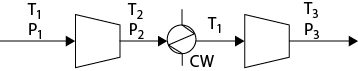
Figure 19.27 Example of Two−Stage Compressor Configuration
19.5.5 Performance of the Feed Section to a Process
A common feature of chemical processes is the mixing of reactant feeds before they enter a reactor. When two streams mix, they are at the same pressure. The consequences of this are illustrated by the following scenario.
Phthalic anhydride can be produced by reacting naphthalene and oxygen. The feed section to a phthalic anhydride process is shown in Figure 19.28. The mixed feed enters a fluidized bed reactor operating at five times the minimum fluidization velocity. A stream table is given in Table 19.4. It is assumed that all frictional pressure losses are associated with equipment and that frictional losses in the piping are negligible. It is temporarily necessary to scale down production by 50%. The engineer must determine how to scale down the process and to determine the new flows and pressures.
)
Figure 19.28 Feed Section to Phthalic Anhydride Process
Table 19.4 Partial Stream Table for Feed Section in Figure 19.27
Stream |
||||||||
1 |
2 |
3 |
4 |
5 |
6 |
7 |
8 |
|
P (kPa) |
80.00 |
101.33 |
343.0 |
268.0 |
243.0 |
243.0 |
243.0 |
200.0 |
Phase |
L |
V |
L |
V |
V |
V |
V |
V |
Naphthalene (Mg/h) |
12.82 |
— |
12.82 |
— |
12.82 |
— |
12.82 |
12.82 |
Air (Mg/h) |
— |
151.47 |
— |
151.47 |
— |
151.47 |
151.47 |
151.47 |
It is necessary to have pump and compressor curves in order to do the required calculations. In this example, equations for the pump curves are used. These equations can be obtained by fitting a polynomial to the curves provided by pump manufacturers. As discussed in Section 19.5.3, pump curves are usually expressed as pressure head versus volumetric flowrate so that they can be used for a liquid of any density. In this example, pressure head and volumetric flowrate have been converted to absolute pressure and mass flowrate using the density of the fluids involved. Pump P-201 operates at only one speed, and an equation for the pump curve is
)
Compressor C-201 operates at only one speed, and the equation for the compressor curve is
)
From Figure 19.27, it is seen that there is only one valve in the feed section, after the mixing point. Therefore, the only way to reduce the production of phthalic anhydride is to close the valve to the point at which the naphthalene feed is reduced by 50%. Example 19.21 illustrates the consequences of reducing the naphthalene feed rate by 50%.
Example 19.21
For a reduction in naphthalene feed by 50%, determine the pressures and flows of all streams after the scale-down.
Solution
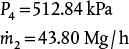
Because it is known that the flowrate of naphthalene has been reduced by 50%, the new outlet pressure from P-201 can be calculated from Equation (19.79). The feed pressure remains at 80 kPa. At a naphthalene flow of 6.41 Mg/h, Equation (19.79) gives a pressure increase of 455.73 kPa, so P3 = 535.73 kPa. Because the flowrate has decreased by a factor of 2, the pressure drop in the fired heater decreases by a factor of 4, since  . Therefore, P5 = 510.73 kPa. Consequently, the pressure of Stream 6 must be 510.73 kPa. The flowrate of air can now be calculated from the compressor curve equation.
The compressor curve equation has two unknowns: the compressor outlet pressure and the mass flowrate. Therefore, a second equation is needed. The second equation is obtained from a base-case ratio for the pressure drop across the heat exchanger. The two equations are
)
)
)
)
)
)
)
)
)
)
)
)
)
)
)
)
The solution is
The stream table for the scaled-down case is given in Table E19.21. Although it is not precisely true, for lack of additional information, it has been assumed that the pressure of Stream 8 remains constant.
Table E19.21 Partial Stream Table for Scaled-Down Feed Section in Figure 19.28
Stream |
||||||||
1 |
2 |
3 |
4 |
5 |
6 |
7 |
8 |
|
P (kPa) |
80.0 |
101.33 |
535.73 |
512.84 |
510.73 |
510.73 |
510.73 |
200.00 |
Phase |
L |
V |
L |
V |
V |
V |
V |
V |
Naphthalene (Mg/h) |
6.41 |
— |
6.41 |
— |
6.41 |
— |
6.41 |
6.41 |
Air (Mg/h) |
— |
43.80 |
— |
43.80 |
— |
43.80 |
43.80 |
43.80 |
It is observed that the flowrate of air is reduced by far more than 50% in the scaled-down case. This is because of the combination of the compressor curve and the new pressure of Streams 5 and 6 after the naphthalene flowrate is scaled down by 50%. The total flowrate of Stream 8 is now 50.21 Mg/h, which is 30.6% of the original flowrate to the reactor. Given that the reactor was operating at five times minimum fluidization, the reactor is now in danger of not being fluidized adequately. Because the phthalic anhydride reaction is very exothermic, a loss of fluidization could result in poor heat transfer, which might result in a runaway reaction. The conclusion is that it is not recommended to operate at these scaled-down conditions.
The question is how the air flowrate can be scaled down by 50% to maintain the same ratio of naphthalene to air as in the original case. The answer is in valve placement. Because of the requirement that the pressures at the mixing point be equal, with only one valve after the mixing point, there is only one possible flowrate of air corresponding to a 50% reduction in naphthalene flow-rate. Effectively, there is no control of the air flowrate. A chemical process would not be designed as in Figure 19.28. The most common design is illustrated in Figure 19.21. With valves in both feed streams, the flowrates of each stream can be controlled independently.
)
Figure E19.21 Feed Section to Phthalic Anhydride Process with Better Valve Placement Than Shown in Figure 19.28