Basic Quantum Theory
- 6.1 Further with Quantum Mechanics
- 6.2 Quantum Decoherence
- 6.3 Quantum Electrodynamics
- 6.4 Quantum Chromodynamics
- 6.5 Feynman Diagram
- 6.6 Summary
- Test Your Skills
This chapter is from the book
This chapter is from the book
This chapter is from the book
Chapter Objectives
After reading this chapter and completing the quizzes, you will be able to do the following:
Use bra-ket notation
Understand the Hamiltonian operator
Have a working knowledge of wave functions and the wave function collapse
Recognize the role of Schrödinger’s equation
Know the role of quantum decoherence and its impact on quantum computing
Have a generalized understanding of quantum electrodynamics
Demonstrate basic knowledge of quantum chromodynamics
This chapter will introduce you to various aspects of quantum theory. Some of these topics were briefly touched on in Chapter 3, “Basic Physics for Quantum Computing.” It is essential that you have a strong grasp of Chapters 1 through 3 in order to follow along in this chapter. The first issue to address is what precisely is quantum theory? It is actually a number of related theories, including quantum field theory, quantum electrodynamics (QED), and in some physicists’ opinion, even quantum chromodynamics, which deals with quarks. In this chapter, the goal is to deepen the knowledge you gained in Chapter 3 and to provide at least a brief introduction to a range of topics that all fit under the umbrella of quantum theory.
In this chapter, it is more important than ever to keep in mind our goal. Yes, I will present a fair amount of mathematics, some of which may be beyond some readers. However, unless your goal is to do actual work in the field of quantum physics or quantum computing research, then what you need is simply a general comprehension of what the equations mean. You do not need to have the level of mathematical acumen that would allow you to actually do the math. So, if you encounter some math you find daunting, simply review it a few times to ensure you get the general gist of it and move on. You can certainly work with qubits, Q#, and other quantum tools later in this book without a deep understanding of how to do the mathematics.
6.1 Further with Quantum Mechanics
Chapter 3 introduced some fundamental concepts in quantum physics. This section expands our exploration of quantum mechanics a bit. In 1932, Werner Heisenberg was awarded the Nobel Prize in Physics for the “creation of quantum mechanics.” I am not sure that one person can be solely credited with the creation of quantum mechanics, but certainly Heisenberg deserves that credit as much as anyone.
The publication that earned him the Nobel Prize was titled “Quantum-Theoretical Re-interpretation of Kinematic and Mechanical Relations.” This paper is rather sophisticated mathematically, and we won’t be exploring it in detail here. The paper introduced a number of concepts that formed the basis of quantum physics. The interested reader can consult several resources, including the following:
https://www.heisenberg-gesellschaft.de/3-the-development-of-quantum-mechanics-1925-ndash-1927.html
https://inis.iaea.org/collection/NCLCollectionStore/_Public/08/282/8282072.pdf
6.1.1 Bra-Ket Notation
Bra-ket notation was introduced a bit earlier, in Chapter 3. However, this notation is so essential to understanding quantum physics and quantum computing that we will revisit it, with more detail. Recall that quantum states are really vectors. These vectors include complex numbers. However, it is often possible to ignore the details of the vector and work with a representation of the vector. This notation is called Dirac notation or bra-ket notation.
A bra is denoted by 〈V|, and a ket is denoted by |V〉. Yes, the terms are intentional, meaning braket, or bracket. But what does this actually mean? A bra describes some linear function that maps each vector in V to a number in the complex plane. Bra-ket notation is really about linear operators on complex vector spaces, and it is the standard way that states are represented in quantum physics and quantum computing. One reason for this notation is to avoid confusion. The term vector in linear algebra is a bit different from the term vector in classical physics. In classical physics, a vector denotes something like velocity that has magnitude and direction; however, in quantum physics, a vector (linear algebra vector) is used to represent a quantum state, thus the need for a different notation. It is important to keep in mind that these are really just vectors. Therefore, the linear algebra that you saw in Chapter 1, “Introduction to Essential Linear Algebra,” applies.
6.1.2 Hamiltonian
It is important that you be introduced to the Hamiltonian. A Hamiltonian is an operator in quantum mechanics. It represents the sum of the kinetic and potential energies (i.e., the total energy) of all the particles in a given system. The Hamiltonian can be denoted by an H, <H>, or  . When one measures the total energy of a system, the set of possible outcomes is the spectrum of the Hamiltonian. The Hamiltonian is named after William Hamilton. As you may surmise, there are multiple different ways of representing the Hamiltonian. In Equation 6.1, you see a simplified version of the Hamiltonian.

EQUATION 6.1 The Hamiltonian
The  represents the kinetic energy, and the
  represents the potential energy. The T is a function of p (the momentum), and V is a function of q (the special coordinate). This simply states that the Hamiltonian is the sum of kinetic and potential energies. This particular formulation is rather simplistic and not overly helpful. It represents a one-dimensional system with one single particle of mass, m. This is a good place to start understanding the Hamiltonian. Equation 6.2 shows a better formulation.
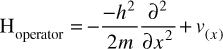
EQUATION 6.2 The Hamiltonian (Detailed)
Let us examine this formula to understand it. The simplest part is V(x), which simply represents potential energy. The x is the coordinate in space. Also rather simple to understand is the m, which is the mass. The  as you will recall from Chapter 3, is the reduced Planck constant, which is the Planck constant h (6.626 × 10⁻³⁴ J⋅s) / 2π. The ∂ symbol indicates a partial derivative. For some readers, this will be quite familiar. If you are not acquainted with derivatives and partial derivatives, you need not master those topics to continue with this book, but a brief conceptual explanation is in order. It should also be noted that there are many other ways of expressing this equation. You can see an alternative way at https://support.dwavesys.com/hc/en-us/articles/360003684614-What-Is-the-Hamiltonian-.
With any function, the derivative of that function is essentially a measurement of the sensitivity of the function’s output with respect to a change in the function’s input. A classic example is calculating an object’s position with respect to change in time, which provides the velocity. A partial derivative is a function of multiple variables, and the derivative is calculated with respect to one of those variables.
So, you should now have a general conceptual understanding of the Hamiltonian. Our previous discussion only concerned a single particle. In a system with multiple particles (as are most systems), the Hamiltonian of the system is just the sum of the individual Hamiltonians, as demonstrated in Equation 6.3.
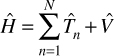
EQUATION 6.3 Hamiltonian (Another View)
Let us delve a bit deeper into the Hamiltonian. Any operator can be written in a matrix form. Now recall our discussion of linear algebra in Chapter 1. The eigenvalues of the Hamiltonian are the energy levels of the system. For the purposes of this book, it is not critical that you understand this at a deep working level, but you should begin to see intuitively why linear algebra is so important for quantum physics.
It also is interesting to note the relationship between the Hamiltonian and the Lagrangian. First, it is necessary to define the Lagrangian. Joseph-Louis Lagrange developed Lagrangian mechanics in 1788. It is essentially a reformulation of classical mechanics. Lagrangian mechanics uses the Lagrangian function of the coordinates, the time derivatives, and the times of the particles.
In Hamiltonian mechanics, the system is described by a set of canonical coordinates. Canonical coordinates are sets of coordinates on a phase space, which can describe a system at any given point in time. You can, in fact, derive the Hamiltonian from a Lagrangian. We won’t delve into that topic in this chapter, but the interested reader can learn more about that process, and other details about the Hamiltonian, at the following sources:
6.1.3 Wave Function Collapse
In physics, a wave function is a mathematical description of the quantum state of a quantum system. It is usually represented by the Greek letter psi, either lowercase (ψ) or uppercase (Ψ). A wave function is a function of the degrees of freedom for the quantum system. In such a system, degrees of freedom indicate the number of independent parameters that describe the system’s state. As one example, photons and electrons have a spin value, and that is a discrete degree of freedom for that particle.
A wave function is a superposition of possible states. More specifically, it is a superposition of eigenstates that collapses to a single eigenstate based on interaction with the environment. Chapter 1 discussed eigenvalues and eigenvectors. An eigenstate is basically what physicists call an eigenvector.
Wave functions can be added together and even multiplied (usually by complex numbers, which you studied in Chapter 2, “Complex Numbers”) to form new wave functions. Recall the dot product we discussed in Chapter 1; the inner product is just another term for the dot product. This is also sometimes called the scalar product. Recall the inner/dot product is easily calculated, as shown in Equation 6.4.

EQUATION 6.4 Inner Product
The inner product of two wave functions is a measure of the overlap between the two wave functions’ physical state.
This brings us to another important aspect of quantum mechanics: the Born rule. This postulate was formulated by Max Born and is sometimes called the Born law or the Born postulate. The postulate gives the probability that a measurement of a quantum system will produce a particular result. The simplest form of this is the probability of finding a particle at a given point. That general description will be sufficient for you to continue in this book; however, if you are interested in a deeper understanding, we will explore it now. The Born rule more specifically states that if some observable (position, momentum, etc.) corresponding to a self-adjoint operator A is measured in a system with a normalized wave function |ψ>, then the result will be one of the eigenvalues of A. This should help you become more comfortable with the probabilistic nature of quantum physics.
For those readers not familiar with self-adjoint operators, a brief overview is provided. Recall from Chapter 1 that matrices are often used as operators. A self-adjoint operator on a finite complex vector space, with an inner product, is a linear map from the vector to itself that is its own adjoint. Note that it is a complex vector space. This bring us to Hermitian. Recall from Chapter 2 that Hermitian refers to a square matrix that is equal to its own conjugate transpose. Conjugate transpose means first taking the transpose of the matrix and then taking the complex conjugate of the matrix. Each linear operator on a complex Hilbert space also has an adjoint operator, sometimes called a Hermitian adjoint.
Self-adjoint operators have applications in fields such as functional analysis; however, in quantum mechanics, physical observables such as position, momentum, spin, and angular momentum are represented by self-adjoint operators on a Hilbert space.
This is also a good time to discuss Born’s rule, which provides the probability that a measurement of a quantum system will yield a particular result. More specifically, the Born rule states that the probability density of finding a particular particle at a specific point is proportional to the square of the magnitude of the particle’s wave function at that point. In more detail, the Born rule states that if an observable corresponding to a self-adjoint operator is measured in a system with a normalized wave function, the result will be one of the eigenvalues of that self-adjoint operator. There are more details to the Born rule, but this should provide you enough information. The interested reader can find more information at the following sources:
Now let us return to the collapse of a wave function, which takes the superposition of possible eigenstates and collapses to a single eigenstate based on interaction with the environment. What is this interaction with the environment? This is one of the aspects of quantum physics that is often misunderstood by the general public. A common interaction with the environment is a measurement, which physicists often describe as an observation. This has led many to associate intelligent observation as a necessary condition for quantum physics, and thus all of reality. That is simply not an accurate depiction of what quantum physics teaches us.
What is termed an observation is actually an interaction with the environment. When a measurement is taken, that is an interaction that causes the wave function to collapse.
The fact that a measurement causes the wave function to collapse has substantial implications for quantum computing. When one measures a particle, one changes the state. As you will see in later chapters, particularly Chapter 8, “Quantum Architecture,” and Chapter 9, “Quantum Hardware,” this is something that quantum computing must account for.
The wave function can be expressed as a linear combination of the eigenstates (recall this is the physics term for eigenvectors you learned in Chapter 1) of an observable (position, momentum, spin, etc.). Using the bra-ket notation discussed previously, this means a wave function has a form such as you see in Equation 6.5.
ψ>=Σici|ϕi
EQUATION 6.5 Wave Function
This is not as complex as it seems. The Greek letter psi (ψ) denotes the wave function. The Σ symbol is a summation of what is after it. The φi represents various possible quantum states. The i is to enumerate through those possible states, such as φ1, φ2, φ3, etc. The ci values (i.e., c1, c2, c3, etc.) are probability coefficients. The letter c is frequently used to denote these because they are represented by complex numbers.
Recall from Chapter 1 that if two vectors are both orthogonal (i.e., perpendicular to each other) and have a unit length (length 1), the vectors are said to be orthonormal. The bra-ket 〈φi|φj 〉 forms an ortho-normal eigenvector basis. This is often written as follows:
〈φi|φj〉 = δij.
The symbol δ is the Kronecker delta, which is a function of two variables. If the variables are equal, the function result is 1. If they are not equal, the function result is 0. This is usually defined as shown in Equation 6.6.
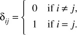
EQUATION 6.6 Kronecker Delta
Now let us discuss the actual process of the wave collapse. Remember that for any observable, the wave function is some linear combination of the eigenbasis before the collapse. When there is some environmental interaction, such as a measurement of the observable, the function collapses to just one of the base’s eigenstates. This can be described in the following rather simple formula:
| ψ〉 → |ϕi〉
But which state will it collapse to? That is the issue with quantum mechanics being probabilistic. We can say that it will collapse to a particular eigenstate |φk〉 with the Born probability (recall we discussed this earlier in this chapter) Pk = |ck|2. The value ck is the probability amplitude for that specific eigenstate. After the measurement, all the other possible eigenstates that are not k have collapsed to 0 (put a bit more mathematically, ci ≠ k = 0).
Measurement has been discussed as one type of interaction with the environment. One of the challenges for quantum computing is that this is not the only type of interaction. Particles interact with other particles. In fact, such things as cosmic rays can interact with quantum states of particles. This is one reason that decoherence is such a problem for quantum computing.
6.1.4 Schrödinger’s Equation
The Schrödinger equation is quite important in quantum physics. It describes the wave function of a quantum system. This equation was published by Erwin Schrödinger in 1926 and resulted in his earning the Nobel Prize in Physics in 1933. First, let us examine the equation itself and ensure you have a general grasp of it; then we can discuss more of its implications. There are various ways to present this equation; we will first examine the time-dependent version. You can see this in Equation 6.7.
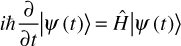
EQUATION 6.7 Schrödinger Equation
Don’t let this overwhelm you. All of the symbols used have already been discussed, and I will discuss them again here to refresh your memory.
Given that we are discussing a time-dependent version of the Schrödinger equation, it should be clear to most readers that the t represents time. Remember that the ∂ symbol indicates a partial derivative. So, we can see in the denominator that there is a partial derivative with respect to time. The  , you will recall from Chapter 3 and from earlier in this chapter, is the reduced Planck constant, which is the Planck constant h (6.626 × 10⁻³⁴ j * s) / 2π. The ψ symbol we saw earlier in this chapter. You may also recall that the symbol Ĥ denotes the Hamiltonian operator, which is the total energy of the particles in a system.
Before we examine the implications of the Schrödinger equation, let us first examine another form of the equation. You can see this in Equation 6.8.
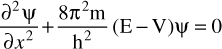
EQUATION 6.8 Schrödinger (Another Form)
You already know that the ∂ symbol indicates a partial derivative. The 2 superposed above it means this is a second derivative (i.e., a derivative of a derivative). For those readers who don’t have a solid calculus background, or who don’t recall their calculus, a second derivative is actually common. A first derivative tells you the rate of change for some function. A second derivative tells you the rate of change for that rate of change that you found in the first derivative. Probably the most common example is acceleration. Speed is the change in position with respect to time. That is the first derivative. Acceleration is the change in speed, which is a second derivative. The ψ symbol denotes the wave function, which you should be getting quite familiar with by now. Another symbol you are familiar with is the h, for Planck’s constant. Note in this form of the Schrödinger equation that it is the Planck constant, not the reduced Planck constant. The E is the kinetic energy, and the V is the potential energy of the system. The X is the position.
Remember that in the subatomic world, we have the issue of wave-particle duality. The Schrödinger equation allows us to calculate how the wave function changes in time.