- 5.1 Frequency-Flat Wireless Channels
- 5.2 Equalization of Frequency-Selective Channels
- 5.3 Estimating Frequency-Selective Channels
- 5.4 Carrier Frequency Offset Correction in Frequency-Selective Channels
- 5.5 Introduction to Wireless Propagation
- 5.6 Large-Scale Channel Models
- 5.7 Small-Scale Fading Selectivity
- 5.8 Small-Scale Channel Models
- 5.9 Summary
- Problems
This chapter is from the book
This chapter is from the book
This chapter is from the book
5.6 Large-Scale Channel Models
In this section, we review several large-scale models for signal strength path loss as a function of distance, denoted by Pr(d). We review the Friis free-space equation as a starting point, followed by the log-distance model and the LOS/NLOS path-loss model. We conclude with some performance calculations using path-loss models.
5.6.1 Friis Free-Space Model
For many propagation prediction models, the starting point has been the Friis free-space model [165, 270]. This model is most appropriate for situations where there are no obstructions present in the propagation environment, like satellite communication links or in millimeter-wave LOS links. The Friis free-space equation is given by

where the key quantities are summarized as follows:
Ptx,lin is the transmit power in linear. For complex pulse-amplitude modulation Ptx,lin = Ex/T.
d is the distance between the transmitter and the receiver. It should be in the same units as λ, normally meters.
λ is the wavelength of the carrier, normally in meters.
Gt,lin and Gr,lin are the transmit and receive antenna gains, normally assumed to be unity unless otherwise given.
A loss factor may also be included in the denominator of (5.276) to account for cable loss, impedance mismatch, and other impairments.
The Friis free-space equation implies that the isotropic path loss (assuming unity antenna gains Gr,lin = Gt,lin = 1) increases inversely with the wavelength squared, λ−2. This fact implies that higher carrier frequencies, which have smaller λ, will have higher path loss. For a given physical antenna aperture, however, the maximum gains for a nonisotropic antenna generally scale as Glin = 4πAe/λ2, where the effective aperture Ae is related to the physical size of the antenna and the antenna design [270]. Therefore, if the antenna aperture is fixed (the antenna area stays “the same size”), then path loss can actually be lower at higher carrier frequencies. Compensating for path loss in this manner, however, requires directional transmission with high-dimensional antenna arrays and is most feasible at higher frequencies like millimeter wave [268].
Most path-loss equations are written in decibels because of the small values involved. Converting the Friis free-space equation into decibels by taking the log of both sides and multiplying by 10 gives

where Prx(d) and Ptx are measured in decibels referenced to 1 watt (dBW) or decibels referenced to 1 milliwatt (dBm), and Gt and Gr are in decibels. All other path-loss equations are given directly in terms of decibels.
The path loss is the ratio of Pr,lin(d) = Ptx,lin/Prx,lin(d), or in decibels Ptx − Prx(d). Path loss is essentially the inverse of the path gain between the transmitter and the receiver. Path loss is used because the inverse of a small gain becomes a large number. The path loss for the Friis free-space equation in decibels is

Example 5.24 Calculate the free-space path loss at 100m assuming Gt = Gr = 0dB and λ = 0.01m.
Answer:

To build intuition, it is instructive to explore what happens as one parameter changes while keeping the other parameters fixed. For example, observe the following (keeping in mind the caveats about how antenna gains might also scale):
If the distance doubles, the path loss increases by 6dB.
If the wavelength doubles, the received power increases by 6dB.
If the frequency doubles (inversely proportional to the wavelength), the received power drops by 6dB.
From a system perspective, it also makes sense to fix the maximum value of loss Pr(d) and then to see how d behaves if other parameters are changed. For example, if the wavelength doubles, then the distance can also be doubled while maintaining the same loss. Equivalently, if the frequency doubles, then the distance decreases by half. This effect is also observed in more complicated real-world propagation settings. For example, with the same power and antenna configuration, a Wi-Fi system operating using 2.4GHz has a longer range than one operating at 5.2GHz. For similar reasons, spectrum in cellular systems below 1GHz is considered more valuable than spectrum above 1GHz (though note that spectrum is very expensive in both cases).
The loss predicted by the free-space equation is optimistic in many terrestrial wireless systems. The reason is that in terrestrial systems, ground reflections and other modes of propagation result in measured powers decreasing more aggressively as a function of distance. This means that the actual received signal power, on average, decays faster than predicted by the free-space equation. There are many other path-loss models inspired by analysis that solve this problem, including the two-ray model or ground bounce model [270], as well as models derived from experimental data like the Okumura [246] or Hata [141] models.
5.6.2 Log-Distance Path-Loss Model
The most common extension of the free-space model is the log-distance path-loss model. This classic model is based on extensive channel measurements. The log-distance path-loss model is

where α and β are the linear parameters and η is a random variable that corresponds to shadowing. The equation is valid for d ≥ d0, where d0 is a reference distance. Often the free-space equation is used for values of d < d0. This results in a two-slope path-loss model, where there may be one distribution of η for d < d0 and another one for d > d0.
The linear model parameters can be chosen to fit measurement data [95, 270]. It is common to select α based on the path loss derived from the free-space equation (5.278) at the reference distance d0. In this way, the α term incorporates the antenna gain and wavelength-dependent effects [312]. A reasonable choice for d0 = 1m; see, for example, [322]. The path-loss exponent is β. Values of β vary a great deal depending on the environment. Values of β < 2 can occur in urban areas or in hallways, in what is called the urban canyon effect. Values of β near 2 correspond to free-space conditions, for example, the LOS link in a millimeter-wave system. Values of β from 3 to as high as 5 are common in microcellular models [56, 282, 107], macrocellular models [141], and indoor WLAN models [96].
The linear portions of the log-distance path-loss model capture the average variation of signal strength as a function of distance and may be called the mean path loss. In measurements, though, there is substantial variation of the measured path loss around the mean path loss. For example, obstruction by buildings creates shadowing. To account for this effect, the random variable η is incorporated. It is common to select η as  . This leads to what is called log-normal shadowing, because η is added in the log domain; in the linear domain log10(η) has a log-normal distribution. The parameter σshad would be determined from measurement data and often has a value around 6 to 8dB. In more elaborate models, it can also be a function of distance. Under the assumption that η is Gaussian, Pr(d) is also Gaussian with mean α + 10β log10(d). For analytical purposes, is common to neglect shadowing and just focus on the mean path loss.
Example 5.25 Calculate the mean log-distance path loss at 100m assuming that β = 4. Compute α from the free-space equation assuming Gt = Gr = 0dB, λ = 0.01m, and reference distance d0 = 1m.
Answer: First, compute the reference distance by finding α = Pr(1) from the free-space equation (5.278):

Second, compute the mean path loss for the given parameters:
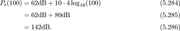
Compared with Example 5.24, there is an additional 40dB of loss due to the higher path-loss exponent in this case.
Example 5.26 Consider the same setup as in Example 5.25. Suppose that the transmit power is Ptx = 20dBm and that σshad = 8dB.
Determine the probability that the received power Prx(100) < −110dBm.
Answer: The received signal power is
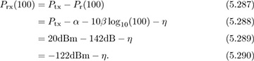
Now note that

where the dBm disappears because dBm − dBm = dB (the 1mW cancels). Now let us rewrite this probability in terms of x ~ N (0, 1):
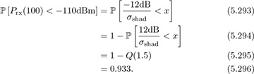
This means that the received power is below −110dBm 93% of the time.
Determine the value of d such that Prx(d) < −110dBm 5% of the time.
Answer: We need to find d such that
 . Following the same steps as in the previous part of the example,
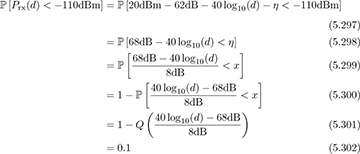
where we recognize that 68dB − 40 log10(d) will be negative, so we can rearrange to get the final answer in the form of a Q-function. Using the inverse of the Q-function gives d = 27.8m.
There are many variations of the log-distance path-loss model, with more refinements based on measurement data and accounting for other parameters. One common model is the COST-231 extended Hata model for use between frequencies of 150MHz and 2GHz. It contains corrections for urban, suburban, and rural environments [336]. The basic equation for path loss in decibels is

where ht is the effective transmitter (base station) antenna height (30m ≤ ht ≤ 200m), hr is the receiver antenna height (1m ≤ hr ≤ 10m), d is the distance between the transmitter and the receiver in kilometers (d ≥ 1km), b(hr) is the correction factor for the effective receiver antenna height, fc is the carrier frequency in megahertz, the parameter C = 0dB for suburban or open environments, and C = 3dB for urban environments. The correction factor is given in decibels as

with other corrections possible for large cities. More realistic path-loss models like COST-231 are useful for simulations but are not as convenient for simple analytical calculations.
5.6.3 LOS/NLOS Path-Loss Model
The log-distance path-loss model accounts for signal blockage using the shadowing term. An alternative approach is to differentiate between blocked (NLOS) and unblocked (LOS) paths more explicitly. This allows each link to be modeled with potentially a smaller error. Such an approach is common in the analysis of millimeter-wave communication systems [20, 344, 13] and has also been used in the 3GPP standards [1, 2].
In the LOS/NLOS path-loss model, there is a distance-dependent probability that an arbitrary link of length d is LOS, which is given by Plos(d). At that same distance, 1 − Plos(d) denotes the probability that the link is NLOS. There are different functions for Plos(d), which depend on the environment. For example,

is used for suburban areas where C = 200m in [1]. For large distances, Plos(d) quickly converges to zero. This matches the intuition that long links are more likely to be blocked.
It is possible to find values of C for any area using concepts from random shape theory [20]. In this case, buildings are modeled as random objects that have independent shape, size, and orientation. For example, assuming the orientation of the buildings is uniformly distributed in space, it follows that

where λbldg is the average number of buildings in a unit area and  is the average perimeter of the buildings in the investigated region. This provides a quick way to approximate the parameters of the LOS probability function without performing extensive simulations and measurements.
Let  denote the path-loss function assuming the link is LOS, and let
  denote the path-loss function assuming the link is NLOS. While any model can be used for these functions, it is common to use the log-distance path-loss model. Shadowing is often not included in the LOS model but may be included in the NLOS model. The path-loss equation is then

where plos(d) is a Bernoulli random variable which is 1 with probability Plos(d), and I(·) is an indicator function that outputs 1 when the argument is true and 0 otherwise. For small values of d the LOS path-loss function dominates, whereas for large values of d the NLOS path-loss function dominates.
Example 5.27 Consider the LOS/NLOS path-loss model. Assume free-space path loss for the LOS term with Gt = Gr = 0dB, λ = 0.01m, and a reference distance d0 = 1m. Assume a log-distance path loss for the NLOS term with β = 4 and α computed from the free-space equation with the same parameters as the LOS function. Assume LOS probability in (5.305) with C = 200m.
Compute the mean signal power at d = 100m.
Answer: First, compute the expectation of (5.307) as

Evaluating at d = 100 and using the results from Example 5.24 and Example 5.25,
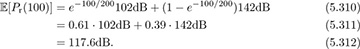
Example 5.28 Consider the same setup as in Example 5.27. Suppose that the transmit power is Ptx = 20dBm. Determine the probability that the received power Prx(100) < −110dBm.
Answer: The received signal power assuming LOS is 20dBm − 102 = −82dBm using the result of Example 5.24. The received power assuming NLOS is 20dBm − 142 = −122dBm using the results of Example 5.25. In the LOS case, the received power is greater than −110dBm, whereas it is less than −110dBm in the NLOS case. Since there is no shadow fading, the probability that the received power Prx(100) < −110dBm is Plos(100) = 0.61.
5.6.4 Performance Analysis Including Path Loss
Large-scale fading can be incorporated into various kinds of performance analysis. To see the impact of path loss on the algorithms proposed in this chapter, a natural approach is to include the G term in (5.275) explicitly when simulating the channel. To illustrate this concept, we consider an AWGN channel, deferring more detailed treatment until after small-scale fading has been introduced.
Consider an AWGN channel where  and G = Ex/Pr,lin(d). The SNR in this case is
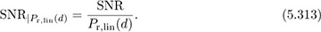
Note that SNRPr,lin(d) may be a random variable if shadowing or blockage is included in the path-loss model. Given a realization of the path loss, the probability of symbol error can then be computed by substituting SNRPr,lin(d) into the appropriate probability of symbol error equation 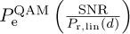 , for example, for M-QAM in (4.147). The average probability of symbol error can be computed by taking the expectation with respect to the random parameters in the path loss as
 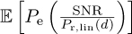 . In some cases, the expectation can be computed exactly. In most cases, though, an efficient way to estimate the average probability of symbol error is through Monte Carlo simulations.
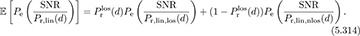
Example 5.29 Compute the average probability of symbol error assuming AWGN and an LOS/NLOS path-loss model.
Answer: Let us denote the path loss in the LOS case as Pr,lin,los(d) and in the NLOS case as Pr,lin,nlos(d), in linear units. Based on (5.307), using similar logic to that in Example 5.27,
Path loss is important for analyzing performance in cellular systems, or more generally any wireless system with frequency reuse. Suppose that a user is located at distance d away from the serving base station. Further suppose that there are Nbs interfering base stations, each a distance dn away from the user. Assuming an AWGN channel, and treating interference as additional noise, the SINR is
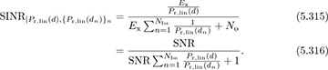
From this expression, it becomes clear that the ratio Pr,lin(d)/Pr,lin(dn) determines the relative significance of the interference. Ideally Pr,lin(d)/Pr,lin(dn) < 1, which means that the user is associated with the strongest base station, even including shadowing or LOS/NLOS effects.