
- Random Numbers and Probability Distributions
- Casino Royale: Roll the Dice
- Normal Distribution
- The Student Who Taught Everyone Else
- Statistical Distributions in Action
- Hypothetically Yours
- The Mean and Kind Differences
- Worked-Out Examples of Hypothesis Testing
- Exercises for Comparison of Means
- Regression for Hypothesis Testing
- Analysis of Variance
- Significantly Correlated
- Summary
This chapter is from the book
This chapter is from the book
This chapter is from the book
The Mean and Kind Differences
We are often concerned with comparing two or more outcomes. For instance, we might be interested in comparing sales from one franchise location with the rest. Statistically, we might have four conditions when we are concerned with comparing the difference in means between groups. These are
- Comparing the sample mean to a population mean when the population standard deviation is known
- Comparing the sample mean to a population mean when the population standard deviation is not known
- Comparing the means of two independent samples with unequal variances
- Comparing the means of two independent samples with equal variances
I discuss each of the four scenarios with examples in the following sections.
Comparing a Sample Mean When the Population SD Is Known
I continue to work with the basketball example. Numerous basketball legends are known for their high-scoring performance. The two in the lead are Wilt Chamberlain and Michael Jordan. However, there appears to be a huge difference between the two leading contenders and others. LeBron James, who is third in the NBA rankings for career average points per game at 27.5, is very much behind Jordan and Chamberlain, and is marginally better than Elgin Baylor at 27.36 (see Figure 6.20).
)
Figure 6.20 Average points scored per game for the leading NBA players
Source: http://www.basketball-reference.com/leaders/pts_per_g_career.html
Many believe that the hefty salaries of celebrity athletes reflect their exceptional performance. In basketball, scoring high points is one of the criteria, among others, that determines a player’s worth. There is some truth to it. During 2013–14, Kobe Bryant of the LA Lakers earned more than $30 million. However, he was not the highest scorer in the team (see Figure 6.21). The basketball example provides us the backdrop to conduct the comparison of means test.
)
Figure 6.21 Lakers: Are they earning their keep?
The Basketball Tryouts
Let us assume that a professional basketball team wants to compare its performance with that of players in a regional league. The pros are known to have a historic mean of 12 points per game with a standard deviation of 5.5. A group of 36 regional players recorded on average 10.7 points per game. The pro coach would like to know whether his professional team scores on average are different from that of the regional players. I will use the two-tailed test from a normal distribution to determine whether the difference is statistically different. I start by calculating the z-value as shown in Equation 6.4:
The specs are as follows:
Average points per player for the regional players: 10.7 ( )
)
Std. Dev of the population: 5.5 (σ)
Average points per game scored by pros: 12 (μ)
Our null hypothesis: H0: μ = 12
Alternative hypothesis: Ha: μ ≠ 12
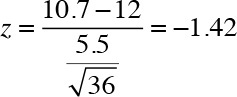
For a two-tailed test at the 5% level, each tail represents 2.5% of the area under the curve. The critical value for the z-test at the 95% level is ±1.96. Because the absolute value for –1.42 is lower than the absolute value for –1.96, I fail to reject the null hypothesis that the difference in means is zero and conclude that statistically speaking, 10.7 is not much different from the pros’ average of 12 points scored per game.
Figure 6.22 presents the z-test graphically. Note that –1.42 does not fall in the gray-shaded area, which constitutes the rejection region. Thus, I cannot reject the null hypothesis that the mean difference is equal to 0.
)
Figure 6.22 Two-tailed test for basketball tryouts
All statistical software and spreadsheets can calculate the p-value associated with the observed mean. In this example using a two-tailed test, the p-value associated with the average score of 10.7 points per game is 0.156, if the mean of the distribution is 12 and the standard error of the mean is 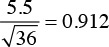
Left Tail Between the Legs
A university basketball team might become a victim of austerity measures. Forced to reduce the budget deficit, the university is considering cutting off underperforming academic and nonacademic programs. The basketball team has not done well as of late. Hence, it has been included in the list of programs to be terminated.
The coach, however, feels that the newly restructured team has the potential to rise to the top of the league and that the bad days are behind them. Disbanding the team now would be a mistake. The coach convinces the university’s vice president of finance to have the team evaluated by a panel of independent coaches to rank the team on a scale of 1 to 10. It was agreed that if the team received the average score of 7 or higher, the team may be allowed to stay for another year, at which time the decision will be revisited.
A panel of 20 independent coaches was assembled to evaluate the team’s performance. After reviewing the team’s performance, the panel’s average score equaled 6.5 with a standard deviation of 1.5. The VP of finance now has to make a decision. Should the team stay or be disbanded?
The VP of finance asked a data analyst in her staff to review the stats and assist her with the decision. She was of the view that the average score of 6.5 was too close to 7, and that she wanted to be sure that there was a statistically significant difference that would prompt her to disband the basketball team.
The analyst decided to conduct a one-sample mean test to determine whether the average score received was 7 or higher.
The null hypothesis: H0: = μ ≥ 7.
The alternative hypothesis: Ha: = μ < 7.
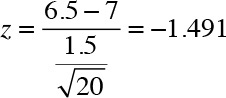
Based on the test, the analyst observed that the z-value of –1.49 does not fall in the rejection region. Thus, he failed to reject the null hypothesis, which stated that the average score received was 7 or higher. The VP of finance, after reviewing the findings, decided not to cut funding to the team because, statistically speaking, the average ranking of the basketball team was not different from the threshold of 7.
The test is graphically illustrated in Figure 6.23.
)
Figure 6.23 Basketball tryouts, left-tail test
Lastly, consider hotdog vendors outside a basketball arena where the local NBA franchise plays. It has been known that when the local team was not winning, the vendors would sell on average 500 hotdogs per game with a standard deviation of 50. Assume now that the home team has been enjoying a winning streak for the last five games that is accompanied with an average sale of 550 hotdogs. The vendors would like to determine whether they are indeed experiencing higher sales. The hypothesis is stated as follows:
The null hypothesis: H0: μ ≤ 500
Alternative hypothesis: Ha: μ > 500
The z-value is calculated as follows:
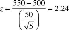
I see that the z-value for the test is 2.24 and the corresponding p-value is 0.0127, which is less than 0.05. I can therefore reject the null hypothesis and conclude that there has been a statistically significant increase in hotdog sales.
Given that I only had five observations, it would have been prudent to use the t-distribution instead, which is more suited to small samples. The test is illustrated in Figure 6.24.
)
Figure 6.24 Hotdog sales
Comparing Means with Unknown Population SD
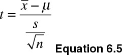
We use the t-distribution in instances where we do not have access to population standard deviation. The test statistic is shown in Equation 6.5:
Note that σ (population standard deviation) has been replaced by s(sample standard deviation).
Consider the case where a large franchise wants to determine the performance of a newly opened store. The franchise surveyed a sample of 35 existing stores and found that the average weekly sales were $166,000 with a standard deviation of $25,000. The new store on average reported a weekly sale of $170,000. The managers behind the launch of the new store are of the view that the new store represents the new approach to retailing, which is the reason why the new store sales are higher than the existing store. Despite their claim of effectively reinventing the science of retailing, the veteran managers maintain that the new store is reporting slightly higher sales because of the novelty factor, which they believe will soon wear off. In addition, they think that statistically speaking, the new store sales are no different from the sample of existing 35 stores.
The question, therefore, is to determine whether the new store sale figures are different from the sales at the existing stores. Because the franchise surveyed 35 of its numerous stores, we do not know the standard deviation of sales in the entire population of stores. Thus, I will rely on t-distribution, and not Normal distribution.
- Average sales per week for the 35 stores: $166,000 (μ)
- Std. Dev of the weekly sales: $25,000 (s)
- Average sales reported by the new store: $170,000 ()
- Our null hypothesis: H0: μ = 166000
- Alternative hypothesis: Ha: μ ≠ 166000
Because we are not making an assumption about the sales in the new store being higher or lower than the average sales in the existing stores, we are using a two-tailed test. The purpose is to test the hypothesis that the new stores sales are different from that of the existing store sales. Mathematically:
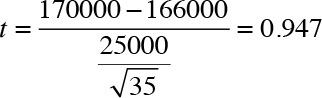
The estimated value of the t-statistics is 0.947. Figure 6.25 shows a graphical representation of the test.
)
Figure 6.25 Retail sales and hypothesis testing
We see that the new store sales do not fall in the rejection region (shaded gray). Furthermore, the p-value for the test is 0.35, which is much higher than the threshold value of 0.05. We therefore fail to reject the null hypothesis and conclude that the new store sales are similar to the ones reported for the 35 sample stores. Thus, the new store manager may not have reinvented the science of retailing.
Comparing Two Means with Unequal Variances
In most applied cases of statistical analysis, we compare the means for two or more groups in a sample. The underlying assumption in this case is that the two means are the same and thus the difference in means equals 0. We can conduct the test assuming the two groups might or might not have equal variances.
I illustrate this concept using data for teaching evaluations and the students’ perceptions of instructors’ appearance. Recall that the data covers information on course evaluations along with course and instructor characteristics for 463 courses for the academic years 2000–2002 at the University of Texas at Austin.
You are encouraged to download the data from the book’s website. A breakdown of male and female instructors’ teaching evaluation scores is presented in Table 6.5.
t.mean<-tapply(x$eval,x$gender, mean)
t.sd<- tapply(x$eval,x$gender, sd)
round(cbind(mean=t.mean, std. dev.=t.sd),2)
Table 6.5 Teaching Evaluation for Male and Female Instructors
mean |
std.dev. |
|
Male |
4.07 |
0.56 |
Female |
3.90 |
0.54 |
We notice that the teaching evaluations of male instructors are slightly higher than that of the female instructors. We would like to know whether this difference is statistically significant.
Hypothesis:
- H0: x1 = x2
- Ha: x1 ≠ x2
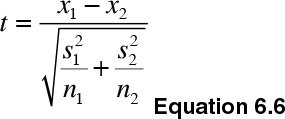
I conduct the test to determine the significance in the difference in average values for a particular characteristic of two independent groups, as shown in Equation 6.6.
The shape of the t-distribution depends on the degrees of freedom, which according to Satterthwaite (1946)5 are calculated as shown in Equation 6.7:
)
Substituting the values in the equation, I have the following:
- s1 = .56
- s2 = .54
- n1 = 268
- n2 = 195
- x1 = 4.07
- x2 = 3.90
Subscript 1 represents statistics for males, and subscript 2 represents statistics for females. The results are as follows: dof = 426 and t = 3.27. The output from R is presented in Figure 6.26.
)
Figure 6.26 Output of a t-test in R
Figure 6.27 shows the graphical output:
)
Figure 6.27 Graphical depiction of a two-tailed t-test for teaching evaluations
I obtain a t-value of 3.27, which falls in the rejection region. I also notice that the p-value for the test is 0.0018, which suggests rejecting the null hypothesis and conclude that the difference in teaching evaluation between male and female instructors is statistically significant at the 95% level.
Conducting a One-Tailed Test
The previous example tested the hypothesis that the average teaching evaluation for males and females was not the same. Now, I adopt a more directional approach and test whether the teaching evaluations for males were higher than that of the females: Ha: x1 > x2.
Given that it is a one-sided test, the only thing that changes from the last iteration is that the rejection region is located only on the right side (see Figure 6.28). The t-value and the associated degrees of freedom remain the same. What changes is the p-value, because the rejection region, representing 5% of the area under the curve, lies to only the right side of the distribution. The probability value will account for the possibility of getting a t-value of 3.27 or higher, which is different from the two-tailed test where I calculated the p-value of obtaining a t-value of either lower than –3.27 or greater than 3.27.
)
Figure 6.28 Teaching evaluations, right-tailed test
The resulting p-value is 0.00058, which is a lot less than 0.05, our chosen threshold to reject the null hypothesis. I thus reject the null and conclude that male instructors indeed receive on average higher teaching evaluations than female instructors do.
Figure 6.29 shows the output from R for a one-tailed test.
)
Figure 6.29 R output for teaching evaluations, right-tailed test
Comparing Two Means with Equal Variances
When the population variance is assumed to be equal between the two groups, the sample variances are pooled to obtain an estimate of σ. Use Equation 6.8 to get the standard deviation of the sampling distribution of the means:
)
Equation 6.9 provides the pooled estimate of variance:
)
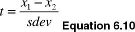
Get the test statistics via Equation 6.10:
I use the same example of teaching evaluations to determine the difference between the evaluation scores of male and female instructors assuming equal variances. The calculations are reported as follows:
)
The degrees of freedom for equal variances are given by dof = n1 + n2 –2.
Figure 6.30 shows the R output:
)
Figure 6.30 R output for equal variances, two-tailed test
Figure 6.31 presents the graphical display.
)
Figure 6.31 Graphical output for equal variances, two-tailed test
Note that the results are similar to what I obtained earlier for the test conducted assuming unequal variances. The t-value is 3.25 and the associated p-value is 0.00124. I reject the null hypothesis and conclude that the average teaching evaluations for males are different from that of the females. These results are statistically significant at the 95% (even 99%) level.
I can repeat the analysis with a one-tailed test to determine whether the teaching evaluations for males are statistically higher than that for females. I report the R output in Figure 6.32. The associated p-value for the one-tailed test is 0.0006194, which suggests rejecting the null hypothesis and conclude that the teaching evaluations for males are greater than that of the females.
)
Figure 6.32 R output for equal variances, right-tailed test
Figure 6.33 shows the graphical display.
)
Figure 6.33 Graphical output for equal variances, right-tailed test