This chapter is from the book
This chapter is from the book
This chapter is from the book
7.2. Generating All Possibilities
Nowhere to go but out,
Nowhere to come but back.
— BEN KING, in The Sum of Life (c. 1893)
Lewis back-tracked the original route up the Missouri.
— LEWIS R. FREEMAN, in National Geographic Magazine (1928)
When you come to one legal road that’s blocked,
you back up and try another.
— PERRY MASON, in The Case of the Black-Eyed Blonde (1944)
7.2.2. Backtrack Programming
Now that we know how to generate simple combinatorial patterns such as tuples, permutations, combinations, partitions, and trees, we’re ready to tackle more exotic patterns that have subtler and less uniform structure. Instances of almost any desired pattern can be generated systematically, at least in principle, if we organize the search carefully. Such a method was christened “backtrack” by R. J. Walker in the 1950s, because it is basically a way to examine all fruitful possibilities while exiting gracefully from situations that have been fully explored.
Most of the patterns we shall deal with can be cast in a simple, general framework: We seek all sequences x1x2 ...xn for which some property Pn(x1,x2,...,xn) holds, where each item xk belongs to some given domain Dk of integers. The backtrack method, in its most elementary form, involves the invention of intermediate “cutoff” properties Pl(x1,...,xl) for 1 ≤ l < n, such that
)
)
(We assume that P0() is always true. Exercise 1 shows that all of the basic patterns studied in Section 7.2.1 can easily be formulated in terms of domains Dk and cutoff properties Pl.) Then we can proceed lexicographically as follows:
Algorithm B (Basic backtrack). Given domains Dk and properties Pl as above, this algorithm visits all sequences x1x2 ...xn that satisfy Pn(x1,x2,...,xn).
B1. [Initialize.] Set l ← 1, and initialize the data structures needed later.
B2. [Enter level l.] (Now Pl−1(x1,...,xl−1) holds.) If l > n, visit x1x2 ...xn and go to B5. Otherwise set xl ← min Dl, the smallest element of Dl.
B3. [Try xl.] If Pl(x1,...,xl) holds, update the data structures to facilitate testing Pl+1, set l ← l + 1, and go to B2.
B4. [Try again.] If xl ≠ max Dl, set xl to the next larger element of Dl and return to B3.
B5. [Backtrack.] Set l ← l−1. If l > 0, downdate the data structures by undoing the changes recently made in step B3, and return to B4. (Otherwise stop.)
The main point is that if Pl(x1,...,xl) is false in step B3, we needn’t waste time trying to append any further values xl+1 ...xn. Thus we can often rule out huge regions of the space of all potential solutions. A second important point is that very little memory is needed, although there may be many, many solutions.
For example, let’s consider the classic problem of n queens: In how many ways can n queens be placed on an n × n board so that no two are in the same row, column, or diagonal? We can suppose that one queen is in each row, and that the queen in row k is in column xk, for 1 ≤ k ≤ n. Then each domain Dk is {1, 2,...,n}; and Pn(x1,...,xn) is the condition that
)
(If xj = xk and j < k, two queens are in the same column; if |xk − xj| = k − j, they’re in the same diagonal.)
This problem is easy to set up for Algorithm B, because we can let property Pl(x1,...,xl) be the same as (3) but restricted to 1 ≤ j < k ≤ l. Condition (1) is clear; and so is condition (2), because Pl requires testing (3) only for k = l when Pl−1 is known. Notice that P1(x1) is always true in this example.
One of the best ways to learn about backtracking is to execute Algorithm B by hand in the special case n = 4 of the n queens problem: First we set x1 ← 1. Then when l = 2 we find P2(1, 1) and P2(1, 2) false; hence we don’t get to l = 3 until trying x2 ← 3. Then, however, we’re stuck, because P3(1, 3,x) is false for 1 ≤ x ≤ 4. Backtracking to level 2, we now try x2 ← 4; and this allows us to set x3 ← 2. However, we’re stuck again, at level 4; and this time we must back up all the way to level 1, because there are no further valid choices at levels 3 and 2. The next choice x1 ← 2 does, happily, lead to a solution without much further ado, namely x1x2x3x4 = 2413. And one more solution (3142) turns up before the algorithm terminates.
The behavior of Algorithm B is nicely visualized as a tree structure, called a search tree or backtrack tree. For example, the backtrack tree for the four queens problem has just 17 nodes,
)
corresponding to the 17 times step B2 is performed. Here xl is shown as the label of an edge from level l − 1 to level l of the tree. (Level l of the algorithm actually corresponds to the tree’s level l − 1, because we’ve chosen to represent patterns using subscripts from 1 to n instead of from 0 to n−1 in this discussion.) The profile (p0,p1,...,pn) of this particular tree — the number of nodes at each level — is (1, 4, 6, 4, 2); and we see that the number of solutions, pn = p4, is 2.
Figure 68 shows the corresponding tree when n = 8. This tree has 2057 nodes, distributed according to the profile (1, 8, 42, 140, 344, 568, 550, 312, 92). Thus the early cutoffs facilitated by backtracking have allowed us to find all 92 solutions by examining only 0.01% of the 88 = 16,777,216 possible sequences x1 ... x8. (And 88 is only 0.38% of the 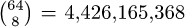 ways to put eight queens on the board.)
7.2.2.1. Dancing links
What a dance do they do Lordy, how I’m tellin’ you!
— HARRY BARRIS, Mississippi Mud (1927)
Don’t lose your confidence if you slip, Be grateful for a pleasant trip, And pick yourself up, dust yourself off, start all over again.
— DOROTHY FIELDS, Pick Yourself Up (1936)
One of the chief characteristics of backtrack algorithms is the fact that they usually need to undo everything that they do to their data structures. In this section we’ll study some extremely simple link-manipulation techniques that modify and unmodify the structures with ease. We’ll also see that these ideas have many, many practical applications.
Suppose we have a doubly linked list, in which each node X has a predecessor and successor denoted respectively by LLINK(X) and RLINK(X). Then we know that it’s easy to delete X from the list, by setting
)
At this point the conventional wisdom is to recycle node X, making it available for reuse in another list. We might also want to tidy things up by clearing LLINK(X) and RLINK(X) to ∧, so that stray pointers to nodes that are still active cannot lead to trouble. (See, for example, Eq. 2.2.5–(4), which is the same as (1) except that it also says ‘AVAIL ⇐ X’.) By contrast, the dancing-links trick resists any urge to do garbage collection. In a backtrack application, we’re better off leaving LLINK(X) and RLINK(X) unchanged. Then we can undo operation (1) by simply setting
)
For example, we might have a 4-element list, as in 2.2.5–(2):
)
If we use (1) to delete the third element, (3) becomes
)
And if we now decide to delete the second element also, we get
)
Exercises—First Set
64. [23] (Clueless jigsaw sudoku.) A jigsaw sudoku puzzle can be called “clueless” if its solution is uniquely determined by the entries in a single row or column, because such clues merely assign names to the n individual symbols that appear. For example, the first such puzzle to be published, discovered in 2000 by Oriel Maxime, is shown here.
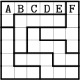
Find all clueless sudoku jigsaw puzzles of order n ≤ 6.
Prove that such puzzles exist of all orders n ≥ 4.
65. [24] Find the unique solutions to the following examples of jigsaw sudoku:
)
▸ 66. [30] Arrange the following sets of nine cards in a 3 × 3 array so that they define a sudoku problem with a unique solution. (Don’t rotate them.)
)
▸ 67. [22] Hypersudoku extends normal sudoku by adding four more (shaded) boxes in which a complete “rainbow” {1, 2, 3, 4, 5, 6, 7, 8, 9} is required to appear:
)
(Such puzzles, introduced by P. Ritmeester in 2005, are featured by many newspapers.)
Show that a hypersudoku solution actually has 18 rainbow boxes, not only 13.
Use that observation to solve hypersudoku puzzles efficiently by extending (30).
How much does that observation help when solving (i) and (ii)?
True or false: A hypersudoku solution remains a hypersudoku solution if the four 4 × 4 blocks that touch its four corners are simultaneously rotated 180°, while also flipping the middle half-rows and middle half-columns (keeping the center fixed).
68. [28] A polyomino is called convex if it contains all of the cells between any two of its cells that lie in the same row or the same column. (This happens if and only if it has the same perimeter as its minimum bounding box does, because each row and column contribute 2.) For example, all of the pentominoes (36) are convex, except for ‘U’.
Generate all ways to pack n convex n-ominoes into an n × n box, for n ≤ 7.
In how many ways can nine convex nonominoes be packed into a 9 × 9 box, when each of them is small enough to fit into a 4 × 4? (Consider also the symmetries.)
▸ 69. [30] Diagram (i) below shows the 81 communities of Bitland, and their nine electoral districts. The voters in each community are either Big-Endian (B) or Little-Endian (L). Each district has a representative in Bitland’s parliament, based on a majority vote.
Notice that there are five Ls and four Bs in every district, hence the parliament is 100% Little-Endian. Everybody agrees that this is unfair. So you have been hired as a computer consultant, to engineer the redistricting.
A rich bigwig secretly offers to pay you a truckload of money if you get the best possible deal for his side. You could gerrymander the districts as in diagram (ii), thereby obtaining seven Big-Endian seats. But that would be too blatantly biased.
)
Show that seven wins for B are actually obtainable with nine districts that do respect the local neighborhoods of Bitland quite decently, because each of them is a convex nonomino that fits in a 4 × 4 square (see exercise 68).
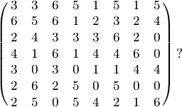
70. [21] Dominosa is a solitaire game in which you “shuffle” the 28 pieces  ,
,  of double-six dominoes and place them at random into a 7 × 8 frame. Then you write down the number of spots in each cell, put the dominoes away, and try to reconstruct their positions based only on that 7 × 8 array of numbers. For example,
)
Show that another placement of dominoes also yields the same matrix of numbers.
What domino placement yields the array
▸ 71. [20] Show that Dominosa reconstruction is a special case of 3D MATCHING.
72. [M22] Generate random instances of Dominosa, and estimate the probability of obtaining a 7 × 8 matrix with a unique solution. Use two models of randomness: (i) Each matrix whose elements are permutations of the multiset {8 × 0, 8 × 1, ..., 8 × 6} is equally likely; (ii) each matrix obtained from a random shuffle of the dominoes is equally likely.
73. [46] What’s the maximum number of solutions to an instance of Dominosa?
Corollary E. Let p1p2 ... pn be any permutation of {1, 2,..., n}. For every signed involution σ that is a symmetry of clauses F, we can write σ in cycle form
)
with i1 ≤ j1, i2 ≤ j2, ... , it ≤ jt, i1 < i2 < … < it, and with 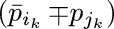 omitted when ik = jk; and we’re allowed to append clauses to F that assert the lexicographic relation
  , where q = t or q is the smallest k with ik = jk.
In the common case when σ is an ordinary signless involution, all of the signs can be eliminated here; we simply assert that  .
.
This involution principle justifies all of the symmetry-breaking techniques that we used above in the pigeonhole and quad-free matrix problems. See, for example, the details discussed in exercise 495.
The idea of breaking symmetry by appending clauses was pioneered by J.-F. Puget [LNCS 689 (1993), 350–361], then by J. Crawford, M. Ginsberg, E. Luks, and A. Roy [Int. Conf. Knowledge Representation and Reasoning 5 (1998), 148–159], who considered unsigned permutations only. They also attempted to discover symmetries algorithmically from the clauses that were given as input. Experience has shown, however, that useful symmetries can almost always be better supplied by a person who understands the structure of the underlying problem.
Indeed, symmetries are often “semantic” rather than “syntactic.” That is, they are symmetries of the underlying Boolean function, but not of the clauses themselves. In the Zarankiewicz problem about quad-free matrices, for example, we appended efficient cardinality clauses to ensure that ∑xij ≥ r; that condition is symmetric under row and column swaps, but the clauses are not.
In this connection it may also be helpful to mention the monkey wrench principle: All of the techniques by which we’ve proved quickly that the pigeonhole clauses are unsatisfiable would have been useless if there had been one more clause such as  ; that clause would have destroyed the symmetry!
We conclude that we’re allowed to remove clauses from F until reaching a subset of clauses F0 for which symmetry-breakers S can be added. If F = F0∪F1, and if F0 is satisfiable ⇔ F0 ∪ S is satisfiable, then F0 ∪ S ⊦ ∈ ⇒ F ⊦ ∈.
One hundred test cases
And now—ta da!—let’s get to the climax of this long story, by looking at how our SAT solvers perform when presented with 100 moderately challenging instances of the satisfiability problem. The 100 sets of clauses summarized on the next two pages come from a cornucopia of different applications, many of which were discussed near the beginning of this section, while others appear in the exercises below.
Every test case has a code name, consisting of a letter and a digit. Table 6 characterizes each problem and also shows exactly how many variables, clauses, and total literals are involved. For example, the description of problem A1 ends with ‘ ’; this means that A1 consists of 24772 clauses on 2043 variables, having 55195 literals altogether, and those clauses are unsatisfiable. Furthermore, since ‘24772’ is underlined, all of A1’s clauses have length 3 or less.
Table 6 Capsule Summaries of The Hundred Test Cases
A1. Find x = x1x2 ... x99 with νx = 27 and no three equally spaced 1s. (See exercise 31.) 2043|24772|55195|U |
A2. Like A1, but x1x2 ... x100. 2071|25197|56147|S |
B1. Cover a mutilated 10 × 10 board with 49 dominoes, without using extra clauses to break symmetry. 176|572|1300|U |
B2. Like B1, but a 12 × 12 board with 71 dominoes. 260|856|1948|U |
C1. Find an 8-step Boolean chain that computes (z2z1z0)2 = x1 + x2 + x3 + x4. (See exercise 479(a).) 384|16944|66336|U |
C2. Find a 7-step Boolean chain that computes the modified full adder functions z1, z2, z3 in exercise 481(b). 469|26637|100063|U |
C3. Like C2, but with 8 steps. 572|33675|134868|S |
C4. Find a 9-step Boolean chain that computes zl and zr in the mod-3 addition problem of exercise 480(b). 678|45098|183834|S |
C5. Connect 1980|22518|70356|S |
C6. Like C5, but move the 1980|22518|70356|U |
C7. Given binary strings s1, ... , s50 of length 200, randomly generated at distances ≤ rj from some string x, find x (see exercise 502). 65719|577368|1659623|S |
C8. Given binary strings s1, ... , s40 of length 500, inspired by biological data, find a string at distance ≤ 42 from each of them. 123540|909120|2569360|U |
C9. Like C8, but at distance ≤ 43. 124100|926200|2620160|S |
D1. Satisfy factor fifo (18, 19, 111111111111). (See exercise 41.) 1940|6374|16498|U |
D2. Like D1, but factor lifo . 1940|6374|16498|U |
D3. Like D1, but (19, 19, 111111111111). 2052|6745|17461|S |
D4. Like D2, but (19, 19, 111111111111). 2052|6745|17461|S |
D5. Solve (x1 ... x9)2 × (y1 ... y9)2 ≠ (x1 ... x9)2 × (y1 ... y9)2, with two copies of the same Dadda multiplication circuit. 864|2791|7236|U |
E0. Find an Erd˝os discrepancy pattern x1 ... x500 (see exercise 482). 1603|9157|27469|S |
E1. Like E0, but x1 ... x750. 2556|14949|44845|S |
E2. Like E0, but x1 ... x1000. 3546|21035|63103|S |
F1. Satisfy fsnark (99). (See exercise 176.) 1782|4161|8913|U |
F2. Like F1, but without the clauses 1782|4159|8909|S |
G1. Win Late Binding Solitaire with the “most difficult winnable deal” in answer 486. 1242|22617|65593|S |
G2. Like G1, but with the most difficult unwinnable deal. 1242|22612|65588|U |
G3. Find a test pattern for the fault “ 3498|11337|29097|S |
G4. Like G3, but for the fault “ 3502|11349|29127|S |
G5. Find a 7 × 15 array X0 leading to X3 = 𝗟𝗜𝗞𝗘 as in Fig. 78, having at most 38 live cells. 7150|28508|71873|U |
G6. Like G5, but at most 39 live cells. 7152|28536|71956|S |
G7. Like G5, but X4 = 𝗟𝗜𝗞𝗘 and X0 can be arbitrary. 8725|33769|84041|U |
G8. Find a configuration in the Game of Life that proves f∗(7, 7) = 28 (see exercise 83). 97909|401836|1020174|S |
K0. Color the 8 × 8 queen graph with 8 colors, using the direct encoding (15) and (16), also forcing the colors of all vertices in the top row. 512|5896|12168|U |
K1. Like K0, but with the exclusion clauses (17) also. 512|7688|15752|U |
K2. Like K1, but with kernel clauses instead of (17) (see answer 14). 512|6408|24328|U |
K3. Like K1, but with support clauses instead of (16) (see exercise 399). 512|13512|97288|U |
K4. Like K1, but using the order encoding for colors. 448|6215|21159|U |
K5. Like K4, but with the hint clauses (162) appended. 448|6299|21663|U |
K6. Like K5, but with double clique hints (exercise 396). 896|8559|27927|U |
K7. Like K1, but with the log encoding of exercise 391(a). 2376|5120|15312|U |
K8. Like K1, but with the log encoding of exercise 391(b). 192|5848|34968|U |
L1. Satisfy langford (10). 130|2437|5204|U |
L2. Satisfy langford′(10). 273|1020|2370|U |
L3. Satisfy langford (13). 228|5875|12356|U |
L4. Satisfy langford′(13). 502|1857|4320|U |
L5. Satisfy langford (32). 1472|102922|210068|S |
L6. Satisfy langford′(32). 3512|12768|29760|S |
L7. Satisfy langford (64). 6016|869650|1756964|S |
L8. Satisfy langford′(64). 14704|53184|124032|S |
M1. Color the McGregor graph of order 10 (Fig. 76) with 4 colors, using one color at most 6 times, via the cardinality constraints (18) and (19). 1064|2752|6244|U |
M2. Like M1, but via (20) and (21). 814|2502|5744|U |
M3. Like M1, but at most 7 times. 1161|2944|6726|S |
M4. Like M2, but at most 7 times. 864|2647|6226|S |
M5. Like M4, but order 16 and at most 11 times. 2256|7801|18756|U |
M6. Like M5, but at most 12 times. 2288|8080|19564|S |
M7. Color the McGregor graph of order 9 with 4 colors, and with at least 18 regions doubly colored (see exercise 19). 952|4539|13875|S |
M8. Like M7, but with at least 19 regions. 952|4540|13877|U |
N1. Place 100 nonattacking queens on a 100 × 100 board. 10000|1151800|2313400|S |
O1. Solve a random open shop scheduling problem with 8 machines and 8 jobs, in 1058 units of time. 50846|557823|1621693|U |
O2. Like O1, but in 1059 units. 50901|558534|1623771|S |
P0. Satisfy (99), (100), and (101) for m = 20, thereby exhibiting a poset of size 20 with no maximal element. 400|7260|22080|U |
P1. Like P0, but with m = 14 and using only the clauses of exercise 228. 196|847|2667|U |
P2. Like P0, but with m = 12 and using only the clauses of exercise 229. 144|530|1674|U |
P3. Like P2, but omitting the clause 144|529|1671|S |
P4. Like P3, but with m = 20. 400|2509|7827|S |
Q0. Like K0, but with 9 colors. 576|6624|13688|S |
Q1. Like K1, but with 9 colors. 576|8928|18296|S |
Q2. Like K2, but with 9 colors. 576|7200|27368|S |
Q3. Like K3, but with 9 colors. 576|15480|123128|S |
Q4. Like K4, but with 9 colors. 512|7008|24200|S |
Q5. Like K5, but with 9 colors. 512|7092|24704|S |
Q6. Like K6, but with 9 colors. 1024|9672|31864|S |
Q7. Like K7, but with 9 colors. 3168|6776|20800|S |
Q8. Like K8, but with 9 colors. 256|6776|52832|S |
Q9. Like Q8, but with the log encoding of exercise 391(c). 256|6584|42256|S |
R1. Satisfy rand (3, 1061, 250, 314159). 250|1061|3183|S |
R2. Satisfy rand (3, 1062, 250, 314159). 250|1062|3186|U |
S1. Find a 4-term disjunctive normal form on {x1,...,x20} that differs from (27) but agrees with it at 108 random training points. 356|4229|16596|S |
S2. Like S1, but at 109 points. 360|4310|16760|U |
S3. Find a sorting network on nine elements that begins with the comparators [1:6][2:7][3:8][4:9] and finishes in five more parallel rounds. (See exercise 64.) 5175|85768|255421|U |
S4. Like S3, but in six more rounds. 6444|107800|326164|S |
T1. Find a 24 × 100 tatami tiling that spells ‘TATAMI’ as in exercise 118. 2874|10527|26112|S |
T2. Like T1, but 24 × 106 and the ‘I’ should have serifs. 3048|11177|27724|U |
T3. Solve the TAOCP problem of exercise 389 with only 4 knight moves. 3752|12069|27548|U |
T4. Like T3, but with 5 knight moves. 3756|12086|27598|S |
T5. Find the pixel in row 5, column 18 of Fig. 80(c), the lexicographically last solution to the Cheshire Tom problem. 8837|39954|100314|S |
T6. Like T5, but column 19. 8837|39955|100315|U |
T7. Solve the run-count extension of the Cheshire Tom problem (see exercise 117). 25734|65670|167263|S |
T8. Like T7, but find a solution that differs from Fig. 79. 25734|65671|167749|U |
W1. Satisfy waerden (3, 10; 97). 97|2779|11662|U |
W2. Satisfy waerden (3, 13; 159). 159|7216|31398|S |
W3. Satisfy waerden (5, 5; 177). 177|7656|38280|S |
W4. Satisfy waerden (5, 5; 178). 178|7744|38720|U |
X1. Prove that the “taking turns” protocol (43) gives mutual exclusion for at least 100 steps. 1010|3612|10614|U |
X2. Prove that assertions Φ for the four-bit protocol of exercise 101, analogous to (50), are invariant. 129|354|926|U |
X3. Prove that Bob won’t starve in 36 steps, assuming the Φ of X2. 1652|10552|28971|U |
X4. Prove that there’s a simple 36-step path with the four-bit protocol, assuming the Φ of X2. 22199|50264|130404|S |
X5. Like X4, but 37 steps. 23388|52822|137034|U |
X6. Like X1, but with Peterson’s protocol (49) instead of (43). 2218|8020|23222|U |
X7. Prove that there’s a simple 54-step path with protocol (49). 26450|56312|147572|S |
X8. Like X7, but 55 steps. 27407|58317|152807|U |
 .
. stuck at 0” in prod (16, 32).
 stuck at 0.”
 .
.)
)
Fig. 95. The clauses of these test cases bind the variables together in significantly different ways. (Illustrations by Carsten Sinz.)
Of course we can’t distinguish hard problems from easy ones by simply counting variables, clauses, and literals. The great versatility with which clauses can capture logical relationships means that different sets of clauses can lead to wildly different phenomena. Some of this immense variety is indicated in Fig. 95, which depicts ten instructive “variable interaction graphs.” Each variable is represented by a ball, and two variables are linked when they appear together in at least one clause. (Some edges are darker than others; see exercise 506. For further examples of such 3D visualizations, presented also in color, see Carsten Sinz, Journal of Automated Reasoning 39 (2007), 219–243.)
A single SAT solver cannot be expected to excel on all of the many species of problems. Furthermore, nearly all of the 100 instances in Table 6 are well beyond the capabilities of the simple algorithms that we began with: Algorithms A, B, and D are unable to crack any of those test cases without needing more than fifty gigamems of computation, except for the simplest examples—L1, L2, L5, P3, P4, and X2. Algorithm L, the souped-up refinement of Algorithm D, also has a lot of difficulty with most of them. On the other hand, Algorithm C does remarkably well. It polishes off 79 of the given problems in fewer than ten Gμ.
Thus the test cases of Table 6 are tough, yet they’re within reach. Almost all of them can be solved in say two minutes, at most, with methods known today.
Complete details can be found in the file SATexamples.tgz on the author’s website, together with many related problems both large and small.
Exactly 50 of these 100 cases are satisfiable. So we’re naturally led to wonder whether Algorithm W (“WalkSAT”) will handle such cases well. The answer is that Algorithm W sometimes succeeds brilliantly—especially on problems C7, C9, L5, L7, M3, M4, M6, P3, P4, Q0, Q1, R1, S1, where it typically outperforms all the other methods we’ve discussed. In particular it solved S1 in just 1 Mμ, in the author’s tests with N = 50n and p = .4, compared to 25 Mμ by the next best method, Algorithm C; it won by 15 Mμ versus Algorithm C’s 83 Mμ on M3, by 83 Mμ versus Algorithm L’s 104 Mμ on Q0, by 95 Mμ versus Algorithm C’s 464 Mμ on Q1, and by a whopping 104 Mμ versus Algorithm C’s 7036 Mμ on C7. That was a surprise. WalkSAT also was reasonably competitive on problem N1. But in all other cases it was nowhere near the method of choice. Therefore we’ll consider only Algorithms L and C in the remainder of this discussion.*
When does a lookahead algorithm like Algorithm L outperform a clause-learning algorithm like Algorithm C? Figure 96 shows how they compare to each other on our 100 test cases: Each problem is plotted with Algorithm C’s running time on the vertical axis and Algorithm L’s on the horizontal axis. Thus Algorithm L is the winner for problems that appear above the dotted line. (This dotted line is “wavy” because times aren’t drawn to scale: The kth fastest running time is shown as k units from the left of the page or from the bottom.)
)
Fig. 96. Comparison of Algorithms C and L on 100 moderately difficult satisfiability problems.
All of these experiments were aborted after 50 Gμ, if necessary, since many of these problems could potentially take centuries before running to completion. Thus the test cases for which Algorithm L timed out appear at the right edge of Fig. 96, and the tough cases for Algorithm C appear at the top. Only E2 and X8 were too hard for both algorithms to handle within the specified cutoff time.
Algorithm L is deterministic: It uses no random variables. However, a slight change (see exercise 505) will randomize it, because the inputs can be shuffled as they are in Algorithm C; and we might as well assume that this change has been made. Then both Algorithms L and C have variable running times. They will find solutions or prove unsatisfiability more quickly on some runs than on others, as we’ve already seen for Algorithm C in Fig. 92.
To compensate for this variability, each of the runtimes reported in Fig. 96 is the median of nine independent trials. Figure 97 shows all 9×100 of the empirical running times obtained with Algorithm C, sorted by their median values. We can see that many of the problems have near-constant behavior; indeed, the ratio max/min was less than 2 in 38 of the cases. But 10 cases turned out to be highly erratic in these experiments, with max/min > 100; problem P4 was actually solved once after only 323 kilomems, while another run lasted 339 gigamems!
One might expect satisfiable problems, such as P4, to benefit more from lucky guesses than unsatisfiable problems do; and these experiments strongly support that hypothesis: Of the 21 problems with max/min > 30, all but P0 are satisfiable, and all 32 of the problems with max/min < 1.7 are unsatisfiable. One might also expect the mean running time (the arithmetic average) to exceed the median running time, in problems like this—because bad luck can be significantly bad, though hopefully rare. Yet the mean is actually smaller than the median in 30 cases, about equally distributed between satisfiable and unsatisfiable.
The median is a nice measure because it is meaningful even in the presence of occasional timeouts. It’s also fair, because we are able to achieve the median time, or better, more often than not.
We should point out that input/output has been excluded from these time comparisons. Each satisfiability problem is supposed to appear within a computer’s memory as a simple list of clauses, after which the counting of mems actually begins. We include the cost of initializing the data structures and solving the problem, but then we stop counting before actually outputting a solution.
Some of the test cases in Table 6 and Fig. 96 represent different encodings of the same problem. For example, problems K0–K8 all demonstrate that the 8 × 8 queen graph can’t be colored with 8 colors. Similarly, problems Q0–Q9 all show that 9 colors will suffice. We’ve already discussed these examples above when considering alternative encodings; and we noted that the best solutions, K6 and Q5, are obtained with an extended order encoding and with Algorithm C. Therefore the fact that Algorithm L beats Algorithm C on problems K0, K1, K2, and K3 is somewhat irrelevant; those problems won’t occur in practice.
Problems L5 and L6 compare different ways to handle the at-most-one constraint. L6 is slightly better for Algorithm L, but Algorithm C prefers L5. Similarly, M1 and M2 compare different ways to deal with a more general cardinality constraint. Here M2 turns out to be better, although both are quite easy for Algorithm C and difficult for Algorithm L.
)
Fig. 97. Nine random running times of Algorithm C, sorted by their medians. (Unsatisfiable cases have solid dots or squares; satisfiable cases are hollow.)
We’ve already noted that Algorithm L shines with respect to random problems such as R1 and R2, and it dominates all competitors even more when unsatisfiable random 3SAT problems get even bigger. Lookahead methods are also successful in waerden problems like W1–W4.
Unsatisfiable Langford problems such as L3 and L4 are definitely bêtes noires for Algorithm C, although not so bad for Algorithm L. Even the world’s fastest CDCL solver, “Treengeling,” was unable to refute the clauses of langford(17) in 2013 until it had learned 26.7 billion clauses; this process took more than a week, using a cluster of 24 computers working together. By contrast, the backtrack method of exercise 7.2.2–21 was able to prove unsatisfiability after fewer than 4Tμ of computation—that’s about 50 minutes on a single vintage-2013 CPU.
We’ve now discussed every case where Algorithm L trounces Algorithm C, except for D5; and D5 is actually somewhat scandalous! It’s an inherently simple problem that hardware designers call a “miter”: Imagine two identical circuits that compute some function f(x1,...,xn), one with gates g1, ... , gm and another with corresponding gates 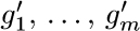 , all represented as in (24). The problem is to find x1 ...xn for which the final results gm and
  aren’t equal. It’s obviously unsatisfiable. Furthermore, there’s an obvious way to refute it, by successively learning the clauses
  ,
,  ,
,  ,
,  , etc. In theory, therefore, Algorithm C will almost surely finish in polynomial time (see exercise 386). But in practice, the algorithm won’t discover those clauses without quite a lot of flailing around, unless special-purpose techniques are introduced to help it discover isomorphic gates.