- Programming Example: Moving to a DL Framework
- The Problem of Saturated Neurons and Vanishing Gradients
- Initialization and Normalization Techniques to Avoid Saturated Neurons
- Cross-Entropy Loss Function to Mitigate Effect of Saturated Output Neurons
- Different Activation Functions to Avoid Vanishing Gradient in Hidden Layers
- Variations on Gradient Descent to Improve Learning
- Experiment: Tweaking Network and Learning Parameters
- Hyperparameter Tuning and Cross-Validation
- Concluding Remarks on the Path Toward Deep Learning
Experiment: Tweaking Network and Learning Parameters
To illustrate the effect of the different techniques, we have defined five different configurations, shown in Table 5-1. Configuration 1 is the same network that we studied in Chapter 4 and at beginning of this chapter. Configuration 2 is the same network but with a learning rate of 10.0. In configuration 3, we change the initialization method to Glorot uniform and change the optimizer to Adam with all parameters taking on the default values. In configuration 4, we change the activation function for the hidden units to ReLU, the initializer for the hidden layer to He normal, and the loss function to cross-entropy. When we described the cross-entropy loss function earlier, it was in the context of a binary classification problem, and the output neuron used the logistic sigmoid function. For multiclass classification problems, we use the categorical cross-entropy loss function, and it is paired with a different output activation known as softmax. The details of softmax are described in Chapter 6, but we use it here with the categorical cross-entropy loss function. Finally, in configuration 5, we change the mini-batch size to 64.
Table 5-1 Configurations with Tweaks to Our Network
CONFIGURATION |
HIDDEN ACTIVATION |
HIDDEN INITIALIZER |
OUTPUT ACTIVATION |
OUTPUT INITIALIZER |
LOSS FUNCTION |
OPTIMIZER |
MINI-BATCH SIZE |
|---|---|---|---|---|---|---|---|
Conf1 |
tanh |
Uniform 0.1 |
Sigmoid |
Uniform 0.1 |
MSE |
SGD lr=0.01 |
1 |
Conf2 |
tanh |
Uniform 0.1 |
Sigmoid |
Uniform 0.1 |
MSE |
SGD lr=10.0 |
1 |
Conf3 |
tanh |
Glorot uniform |
Sigmoid |
Glorot uniform |
MSE |
Adam |
1 |
Conf4 |
ReLU |
He normal |
Softmax |
Glorot uniform |
CE |
Adam |
1 |
Conf5 |
ReLU |
He normal |
Softmax |
Glorot uniform |
CE |
Adam |
64 |
Note: CE, cross-entropy; MSE, mean squared error; SGD, stochastic gradient descent.
Modifying the code to model these configurations is trivial using our DL framework. In Code Snippet 5-13, we show the statements for setting up the model for configuration 5, using ReLU units with He normal initialization in the hidden layer and softmax units with Glorot uniform initialization in the output layer. The model is then compiled using categorical cross-entropy as the loss function and Adam as the optimizer. Finally, the model is trained for 20 epochs using a mini-batch size of 64 (set to BATCH_SIZE=64 in the init code).
Code Snippet 5-13 Code Changes Needed for Configuration 5
model = keras.Sequential([
    keras.layers.Flatten(input_shape=(28, 28)),
    keras.layers.Dense(25, activation='relu',
                       kernel_initializer='he_normal',
                       bias_initializer='zeros'),
    keras.layers.Dense(10, activation='softmax',
                       kernel_initializer='glorot_uniform',
                       bias_initializer='zeros')])

model.compile(loss='categorical_crossentropy',
                    optimizer = 'adam',
                    metrics =['accuracy'])

history = model.fit(train_images, train_labels,
                    validation_data=(test_images, test_labels),
                    epochs=EPOCHS, batch_size=BATCH_SIZE,
                    verbose=2, shuffle=True)
If you run this configuration on a GPU-accelerated platform, you will notice that it is much faster than the previous configuration. The key here is that we have a batch size of 64, which results in 64 training examples being computed in parallel, as opposed to the initial configuration where they were all done serially.
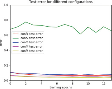
The results of the experiment are shown in Figure 5-12, which shows how the test errors for all configurations evolve during the training process.

FIGURE 5-12 Error on the test dataset for the five configurations
Configuration 1 (red line) ends up at an error of approximately 6%. We spent a nontrivial amount of time on testing different parameters to come up with that configuration (not shown in this book).
Configuration 2 (green) shows what happens if we set the learning rate to 10.0, which is significantly higher than 0.01. The error fluctuates at approximately 70%, and the model never learns much.
Configuration 3 (blue) shows what happens if, instead of using our tuned learning rate and initialization strategy, we choose a “vanilla configuration” with Glorot initialization and the Adam optimizer with its default values. The error is approximately 7%.
For Configuration 4 (purple), we switch to using different activation functions and the cross-entropy error function. We also change the initializer for the hidden layer to He normal. We see that the test error is reduced to 5%.
For Configuration 5 (yellow), the only thing we change compared to Configuration 4 is the mini-batch size: 64 instead of 1. This is our best configuration, which ends up with a test error of approximately 4%. It also runs much faster than the other configurations because the use of a mini-batch size of 64 enables more examples to be computed in parallel.
Although the improvements might not seem that impressive, we should recognize that reducing the error from 6% to 4% means removing one-third of the error cases, which definitely is significant. More important, the presented techniques enable us to train deeper networks.
