CUDA for Engineers: 2D Grids and Interactive Graphics

This chapter is from the book

CUDA for Engineers: An Introduction to High-Performance Parallel Computing

Learn More Buy

This chapter is from the book

This chapter is from the book 

CUDA for Engineers: An Introduction to High-Performance Parallel Computing

Learn More Buy

Application: Stability

To drive home the idea of using the flashlight app as a template for creating more interesting and useful apps, let’s do exactly that. Here we build on flashlight to create an app that analyzes the stability of a linear oscillator, and then we extend the app to handle general single degree of freedom (1DoF) systems, including the van der Pol oscillator, which has more interesting behavior.

The linear oscillator arises from models of a mechanical mass-spring-damper system, an electrical RLC circuit, and the behavior of just about any 1DoF system in the vicinity of an equilibrium point. The mathematical model consists of a single second-order ordinary differential equation (ODE) that can be written in its simplest form (with suitable choice of time unit) as x” + 2bx’ + x = 0, where x is the displacement from the equilibrium position, b is the damping constant, and the primes indicate time derivatives. To put things in a handy form for finding solutions, we convert to a system of two first-order ODEs by introducing the velocity y as a new variable and writing the first-order ODEs that give the rate of change of x and y:

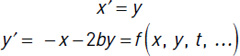
As a bit of foreshadowing, everything we do from here generalizes to a wide variety of 1DoF oscillators by just plugging other expressions in for f(x, y, t, ...) on the right-hand side of the y-equation. While we can write analytical solutions for the linear oscillator, here we focus on numerical solutions using finite difference methods that apply to the more general case. Finite difference methods compute values at discrete multiples of the time step dt (so we introduce t_k = k * dt, x_k = x(t_k), and y_k = y(t_k) as the relevant variables) and replace exact derivatives by difference approximations; that is, x′ → (x_k+1 – x_k) / dt, y′ → (y_k+1 – y_k) / dt. Here we apply the simplest finite difference approach, the explicit Euler method, by substituting the finite difference expressions for the derivatives and solving for the new values at the end of the time step, x_k+1 and y_k+1, in terms of the previous values at the beginning of a time step, x_k and y_k, to obtain:

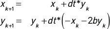
We can then choose an initial state {x_o, y_o} and compute the state of the system at successive time steps.

We’ve just described a method for computing a solution (a sequence of states) arising from a single initial state, and the solution method is completely serial: Entries in the sequence of states are computed one after another.

However, stability depends not on the solution for one initial state but on the solutions for all initial states. For a stable equilibrium, all nearby initial states produce solutions that approach (or at least don’t get further from) the equilibrium. Finding a solution that grows away from the equilibrium indicates instability. For more information on dynamics and stability, see ^7,8.

It is this collective-behavior aspect that makes stability testing such a good candidate for parallelization: By launching a computational grid with initial states densely sampling the neighborhood of the equilibrium, we can test the solutions arising from the surrounding initial states. We’ll see that we can compute hundreds of thousands of solutions in parallel and, with CUDA/OpenGL interop, see and interact with the results in real time.

In particular, we’ll choose a grid of initial states that regularly sample a rectangle centered on the equilibrium. We’ll compute the corresponding solutions and assign shading values based on the fractional change in distance, dist_r (for distance ratio) from the equilibrium during the simulation. To display the results, we’ll assign each pixel a red channel value proportional to the distance ratio (and clipped to [0, 255]) and a blue channel value proportional to the inverse distance ratio (and clipped). Initial states producing solutions that are attracted to the equilibrium (and suggest stability) are dominated by blue, while initial states that produce solutions being repelled from the equilibrium are dominated by red, and the attracting/repelling transition is indicated by equal parts of blue and red; that is, purple.

The result shown in the graphics window will then consist of the equilibrium (at the intersection of the horizontal x-axis and the vertical y-axis shown using the green channel) on a field of red, blue, or purple pixels. Figure 4.3 previews a result from the stability application with both attracting and repelling regions.

Figure 4.3 Stability map with shading adjusted to show a bright central repelling region and surrounding darker attracting region

We now have a plan for producing a stability image for a single system, but we will also introduce interactions so we can observe how the stability image changes for different parameter values or for different systems.

With the plan for the kernel and the interactions in mind, we are ready to look at the code. As promised, the major changes from the flashlight app involve a new kernel function (and a few supporting functions), as shown in Listing 4.10, and new interactivity specifications, as shown in Listing 4.11.

Listing 4.10 stability/kernel.cu

  1 #include "kernel.h"
  2 #define TX 32
  3 #define TY 32
  4 #define LEN 5.f
  5 #define TIME_STEP 0.005f
  6 #define FINAL_TIME 10.f
  7
  8 // scale coordinates onto [-LEN, LEN]
  9 __device__
 10 float scale(int i, int w) { return 2*LEN*(((1.f*i)/w) - 0.5f); }
 11
 12 // function for right-hand side of y-equation
 13 __device__
 14 float f(float x, float y, float param, float sys) {
 15   if (sys == 1) return x - 2*param*y; // negative stiffness
 16   if (sys == 2) return -x + param*(1 - x*x)*y; //van der Pol
 17   else return -x - 2*param*y;
 18 }
 19
 20 // explicit Euler solver
 21 __device__
 22 float2 euler(float x, float y, float dt, float tFinal,
 23              float param, float sys) {
 24   float dx = 0.f, dy = 0.f;
 25   for (float t = 0; t < tFinal; t += dt) {
 26     dx = dt*y;
 27     dy = dt*f(x, y, param, sys);
 28     x += dx;
 29     y += dy;
 30   }
 31   return make_float2(x, y);
 32 }
 33
 34 __device__
 35 unsigned char clip(float x){ return x > 255 ? 255 : (x < 0 ? 0 : x); }
 36
 37 // kernel function to compute decay and shading
 38 __global__
 39 void stabImageKernel(uchar4 *d_out, int w, int h, float p, int s) {
 40   const int c = blockIdx.x*blockDim.x + threadIdx.x;
 41   const int r = blockIdx.y*blockDim.y + threadIdx.y;
 42   if ((c >= w) || (r >= h)) return; // Check if within image bounds
 43   const int i = c + r*w; // 1D indexing
 44   const float x0 = scale(c, w);
 45   const float y0 = scale(r, h);
 46   const float dist_0 = sqrt(x0*x0 + y0*y0);
 47   const float2 pos = euler(x0, y0, TIME_STEP, FINAL_TIME, p, s);
 48   const float dist_f = sqrt(pos.x*pos.x + pos.y*pos.y);
 49   // assign colors based on distance from origin
 50   const float dist_r = dist_f/dist_0;
 51   d_out[i].x = clip(dist_r*255); // red ~ growth
 52   d_out[i].y = ((c == w/2) || (r == h/2)) ? 255 : 0; // axes
 53   d_out[i].z = clip((1/dist_r)*255); // blue ~ 1/growth
 54   d_out[i].w = 255;
 55 }
 56
 57 void kernelLauncher(uchar4 *d_out, int w, int h, float p, int s) {
 58   const dim3 blockSize(TX, TY);
 59   const dim3 gridSize = dim3((w + TX - 1)/TX, (h + TY - 1)/TY);
 60   stabImageKernel<<<gridSize, blockSize>>>(d_out, w, h, p, s);
 61 }

Here is a brief description of the code in kernel.cu. Lines 1–6 include kernel.h and define constant values for thread counts, the spatial scale factor, and the time step and time interval for the simulation. Lines 8–35 define new device functions that will be called by the kernel:

• scale() scales the pixel values onto the coordinate range [-LEN, LEN].

• f() gives the rate of change of the velocity. If you are interested in studying other 1DoF oscillators, you can edit this to correspond to your system of interest. In the sample code, three different versions are included corresponding to different values of the variable sys.

  • The default version with sys = 0 is the damped linear oscillator discussed above.
  • Setting sys = 1 corresponds to a linear oscillator with negative effective stiffness (which may seem odd at first, but that is exactly the case near the inverted position of a pendulum).
  • Setting sys = 2 corresponds to a personal favorite, the van der Pol oscillator, which has a nonlinear damping term.
• euler() performs the simulation for a given initial state and returns a float2 value corresponding to the location of the trajectory at the end of the simulation interval. (Note that the float2 type allows us to bundle the position and velocity together into a single entity. The alternative approach, passing a pointer to memory allocated to store multiple values as we do to handle larger sets of output from kernel functions, is not needed in this case.)

Lines 34–35 define the same clip() function that we used in the flashlight app, and the definition of the new kernel, stabImageKernel(), starts on line 38. Note that arguments have been added for the damping parameter value, p, and the system specifier, s. The index computation and bounds checking in lines 40–43 is exactly as in distanceKernel() from the flashlight app. On lines 44–45 we introduce {x0, y0} as the scaled float coordinate values (which range from –LEN to LEN) corresponding to the pixel location and compute the initial distance, dist_0, from the equilibrium point at the origin. Line 47 calls euler() to perform the simulation with fixed time increment TIME_STEP over an interval of duration FINAL_TIME and return pos, the state the simulated trajectory has reached at the end of the simulation. Line 50 compares the final distance from the origin and to the initial distance. Lines 51–54 assign shading values based on the distance comparison with blue indicating decay toward equilibrium (a.k.a. a vote in favor of stability) and red indicating growth away from equilibrium (which vetoes other votes for stability). Line 52 uses the green channel to show the horizontal x-axis and the vertical y-axis which intersect at the equilibrium point.

Lines 57–61 define the revised wrapper function kernelLauncher() with the correct list of arguments and name of the kernel to be launched.

Listing 4.11 stability/interactions.h

  1 #ifndef INTERACTIONS_H
  2 #define INTERACTIONS_H
  3 #define W 600
  4 #define H 600
  5 #define DELTA_P 0.1f
  6 #define TITLE_STRING "Stability"
  7 int sys = 0;
  8 float param = 0.1f;
  9 void keyboard(unsigned char key, int x, int y) {
 10   if (key == 27)  exit(0);
 11   if (key == '0') sys = 0;
 12   if (key == '1') sys = 1;
 13   if (key == '2') sys = 2;
 14   glutPostRedisplay();
 15 }
 16
 17 void handleSpecialKeypress(int key, int x, int y) {
 18   if (key == GLUT_KEY_DOWN) param -= DELTA_P;
 19   if (key == GLUT_KEY_UP)   param += DELTA_P;
 20   glutPostRedisplay();
 21 }
 22
 23 // no mouse interactions implemented for this app
 24 void mouseMove(int x, int y) { return; }
 25 void mouseDrag(int x, int y) { return; }
 26
 27 void printInstructions() {
 28   printf("Stability visualizer\n");
 29   printf("Use number keys to select system:\n");
 30   printf("\t0: linear oscillator: positive stiffness\n");
 31   printf("\t1: linear oscillator: negative stiffness\n");
 32   printf("\t2: van der Pol oscillator: nonlinear damping\n");
 33   printf("up/down arrow keys adjust parameter value\n\n");
 34   printf("Choose the van der Pol (sys=2)\n");
 35   printf("Keep up arrow key depressed and watch the show.\n");
 36 }
 37
 38 #endif

The description of the alterations to interactions.h, as shown in Listing 4.11, is also straightforward. To the #define statements that set the width W and height H of the image, we add DELTA_P for the size of parameter value increments. Lines 7–8 initialize variables for the system identifier sys and the parameter value param, which is for adjusting the damping value.

There are a few keyboard interactions: Pressing Esc exits the app; pressing number key 0, 1, or 2 selects the system to simulate; and the up arrow and down arrow keys decrease or increase the damping parameter value by DELTA_P. There are no planned mouse interactions, so mouseMove() and mouseDrag() simply return without doing anything.

Finally, there are a couple details to take care of in other files:

• kernel.h contains the prototype for kernelLauncher(), so the first line of the function definition from kernel.cu should be copied and pasted (with a colon terminator) in place of the old prototype in flashlight/kernel.h.

• A couple small changes are also needed in main.cpp:

  • The argument list for the kernelLauncher() call in render() has changed, and that call needs to be changed to match the syntax of the revised kernel.
  • render() is also an appropriate place for specifying information to be displayed in the title bar of the graphics window. For example, the sample code displays an application name (“Stability”) followed by the values of param and sys. Listing 4.12 shows the updated version of render() with the title bar information and updated kernel launch call.

Listing 4.12 Updated render() function for stability/main.cpp

  1 void render() {
  2   uchar4 *d_out = 0;
  3   cudaGraphicsMapResources(1, &cuda_pbo_resource, 0);
  4   cudaGraphicsResourceGetMappedPointer((void **)&d_out, NULL,
  5                                        cuda_pbo_resource);
  6   kernelLauncher(d_out, W, H, param, sys);
  7   cudaGraphicsUnmapResources(1, &cuda_pbo_resource, 0);
  8   // update contents of the title bar
  9   char title[64];
 10   sprintf(title, "Stability: param = %.1f, sys = %d", param, sys);
 11   glutSetWindowTitle(title);
 12 }

Running the Stability Visualizer

Now that we’ve toured the relevant code, it is time to test out the app. In Linux, the Makefile for building this project is the same as the Makefile for the flashlight app that was provided in Listing 4.9. In Visual Studio, the included library files and the project settings are the same as described in flashlight. When you build and run the application, two windows should open: the usual command window showing a brief summary of supported user inputs and a graphics window showing the stability results. The default settings specify the linear oscillator with positive damping, which you can verify from the title bar that displays Stability: param = 0.1, sys = 0, as shown in Figure 4.4(a). Since all solutions of an unforced, damped linear oscillator are attracted toward the equilibrium, the graphics window should show the coordinate axes on a dark field, indicating stability. Next you might test the down arrow key. A single press reduces the damping value from 0.1 to 0.0 (which you should be able to verify in the title bar), and you should see the field changes from dark to moderately bright, as shown in Figure 4.4(b). The linear oscillator with zero damping is neutrally stable (with sinusoidal oscillations that remain near, but do not approach, the equilibrium). The explicit Euler ODE solver happens to produce small errors that systematically favor repulsion from the origin, but the color scheme correctly indicates that all initial states lead to solutions that roughly maintain their distance from the equilibrium. Another press of the down arrow key changes the damping parameter value to −0.1, and the bright field shown in Figure 4.4(c) legitimately indicates instability.

Figure 4.4 Stability visualization for the linear oscillator with different damping parameter values. (a) For param = 0.1, the dark field indicates solutions attracted to a stable equilibrium. (b) For param = 0.0, the moderately bright field indicates neutral stability. (c) For param = -0.1, the bright field indicates solutions repelled from an unstable equilibrium.

Now press the 1 key to set sys = 1 corresponding to a system with negative effective stiffness, and increase the damping value. You should now see the axes on a bright field with a dark sector (and moderately bright transition regions), as shown in Figure 4.5. In this case, some solutions are approaching the equilibrium, but almost all initial conditions lead to solutions that grow away from the equilibrium, which is unstable.

Figure 4.5 Phase plane of a linear oscillator with negative stiffness. A dark sector appears, but the bright field indicates growth away from an unstable equilibrium.

Setting the damping param = 0.0 and sys = 2 brings us to the final case in the example, the van der Pol oscillator. With param = 0.0, this system is identical to the undamped linear oscillator, so we again see the equilibrium in a moderately bright field. What happens when you press the up arrow key to make the damping positive? The equilibrium is surrounded by a bright region, so nearby initial states produce solutions that are repelled and the equilibrium is unstable. However, the outer region is dark, so initial states further out produce solutions that are attracted inwards. There is no other equilibrium point to go to, so where do all these solutions end up? It turns out that there is a closed, attracting loop near the shading transition corresponding to a stable period motion or “limit cycle” (Figure 4.6).

Figure 4.6 Phase plane of the van der Pol oscillator. The bright central region indicates an unstable equilibrium. The dark outer region indicates solutions decaying inwards. These results are consistent with the existence of a stable periodic “limit cycle” trajectory in the moderately bright region.

Note that the results of this type of numerical stability analysis should be considered as advisory. The ODE solver is approximate, and we only test a few hundred thousand initial states, so it is highly likely but not guaranteed that we did not miss something.

Before we are done, you might want to press and hold the up arrow key and watch the hundreds of thousands of pixels in the stability visualization change in real time. This is something you are not likely to be able to do without the power of parallel computing.