This chapter is from the book
This chapter is from the book
This chapter is from the book
15.6. Rasterization
We now move on to implement the rasterizing renderer, and compare it to the ray-casting renderer, observing places where each is more efficient and how the restructuring of the code allows for these efficiencies. The relatively tiny change turns out to have substantial impact on computation time, communication demands, and cache coherence.
15.6.1. Swapping the Loops
Listing 15.22 shows an implementation of rasterize that corresponds closely to rayTrace with the nesting order inverted. The immediate implication of inverting the loop order is that we must store the distance to the closest known intersection at each pixel in a large buffer (depthBuffer), rather than in a single float. This is because we no longer process a single pixel to completion before moving to another pixel, so we must store the intermediate processing state. Some implementations store the depth as a distance along the z-axis, or as the inverse of that distance. We choose to store distance along an eye ray to more closely match the ray-caster structure.
The same intermediate state problem arises for the ray R. We could create a buffer of rays. In practice, the rays are fairly cheap to recompute and don’t justify storage, and we will soon see alternative methods for eliminating the per-pixel ray computation altogether.
Listing 15.22: Rasterizer implemented by simply inverting the nesting order of the loops from the ray tracer, but adding a DepthBuffer.
1voidrasterize(Image& image,constScene& scene,constCamera& camera){ 2 3const intw = image.width(), h = image.height(); 4 DepthBuffer depthBuffer(w, h, INFINITY); 5 6// For each triangle7for(unsigned intt = 0; t < scene.triangleArray.size(); ++t) { 8constTriangle& T = scene.triangleArray[t]; 9 10// Very conservative bounds: the whole screen11const intx0 = 0; 12const intx1 = w; 13 14const inty0 = 0; 15const inty1 = h; 16 17// For each pixel18for(inty = y0; y < y1; ++y) { 19for(intx = x0; x < x1; ++x) { 20constRay& R = computeEyeRay(x, y, w, h, camera); 21 22Radiance3L_o; 23floatdistance = depthBuffer.get(x, y); 24if(sampleRayTriangle(scene, x, y, R, T, L_o, distance)) { 25 image.set(x, y, L_o); 26 depthBuffer.set(x, y, distance); 27 } 28 } 29 } 30 } 31 }
The DepthBuffer class is similar to Image, but it stores a single float at each pixel. Buffers over the image domain are common in computer graphics. This is a good opportunity for code reuse through polymorphism. In C++, the main polymorphic language feature is the template, which corresponds to templates in C# and generics in Java. One could design a templated Buffer class and then instantiate it for Radiance3, float, or whatever per-pixel data was desired. Since methods for saving to disk or gamma correction may not be appropriate for all template parameters, those are best left to subclasses of a specific template instance.
For the initial rasterizer implementation, this level of design is not required. You may simply implement DepthBuffer by copying the Image class implementation, replacing Radiance3 with float, and deleting the display and save methods. We leave the implementation as an exercise.
After implementing Listing 15.22, we need to test the rasterizer. At this time, we trust our ray tracer’s results. So we run the rasterizer and ray tracer on the same scene, for which they should generate identical pixel values. As before, if the results are not identical, then the differences may give clues about the nature of the bug.
15.6.2. Bounding-Box Optimization
So far, we implemented rasterization by simply inverting the order of the for-each-triangle and for-each-pixel loops in a ray tracer. This performs many ray-triangle intersection tests that will fail. This is referred to as poor sample test efficiency.
We can significantly improve sample test efficiency, and therefore performance, on small triangles by only considering pixels whose centers are near the projection of the triangle. To do this we need a heuristic for efficiently bounding each triangle’s projection. The bound must be conservative so that we never miss an intersection. The initial implementation already used a very conservative bound. It assumed that every triangle’s projection was “near” every pixel on the screen. For large triangles, that may be true. For triangles whose true projection is small in screen space, that bound is too conservative.
The best bound would be a triangle’s true projection, and many rasterizers in fact use that. However, there are significant amounts of boilerplate and corner cases in iterating over a triangular section of an image, so here we will instead use a more conservative but still reasonable bound: the 2D axis-aligned bounding box about the triangle’s projection. For a large nondegenerate triangle, this covers about twice the number of pixels as the triangle itself.
The axis-aligned bounding box, however, is straightforward to compute and will produce a significant speedup for many scenes. It is also the method favored by many hardware rasterization designs because the performance is very predictable, and for very small triangles the cost of computing a more accurate bound might dominate the ray-triangle intersection test.
The code in Listing 15.23 determines the bounding box of a triangle T. The code projects each vertex from the camera’s 3D reference frame onto the plane z = –1, and then maps those vertices into the screen space 2D reference frame. This operation is handled entirely by the perspectiveProject helper function. The code then computes the minimum and maximum screen-space positions of the vertices and rounds them (by adding 0.5 and then casting the floating-point values to integers) to integer pixel locations to use as the for-each-pixel bounds.
The interesting work is performed by perspectiveProject. This inverts the process that computeEyeRay performed to find the eye-ray origin (before advancing it to the near plane). A direct implementation following that derivation is given in Listing 15.24. Chapter 13 gives a derivation for this operation as a matrix-vector product followed by a homogeneous division operation. That implementation is more appropriate when the perspective projection follows a series of other transformations that are also expressed as matrices so that the cost of the matrix-vector product can be amortized over all transformations. This version is potentially more computationally efficient (assuming that the constant subexpressions are precomputed) for the case where there are no other transformations; we also give this version to remind you of the derivation of the perspective projection matrix.
Listing 15.23: Projecting vertices and computing the screen-space bounding box.
1Vector2low(image.width(), image.height()); 2Vector2high(0, 0); 3 4for(intv = 0; v < 3; ++v) { 5constVector2& X = perspectiveProject(T.vertex(v), image.width (), image.height(), camera); 6 high = high.max(X); 7 low = low.min(X); 8 } 9 10const intx0 = (int)(low.x + 0.5f); 11const intx1 = (int)(high.x + 0.5f); 12 13const inty0 = (int)(low.y + 0.5f); 14const inty1 = (int)(high.y + 0.5f);
Listing 15.24: Perspective projection.
1Vector2perspectiveProject(constVector3& P,intwidth,intheight, 2constCamera& camera) {// Project onto z = -13Vector2Q(-P.x / P.z, -P.y / P.z); 4 5const floataspect = float(height) / width; 6 7// Compute the side of a square at z = -1 based on our8// horizontal left-edge-to-right-edge field of view9const floats = -2.0f * tan(camera.fieldOfViewX * 0.5f); 10 11 Q.x = width * (-Q.x / s + 0.5f); 12 Q.y = height * (Q.y / (s * aspect) + 0.5f); 13 14returnQ; 15 }
Integrate the listings from this section into your rasterizer and run it. The results should exactly match the ray tracer and simpler rasterizer. Furthermore, it should be measurably faster than the simple rasterizer (although both are likely so fast for simple scenes that rendering seems instantaneous).
Simply verifying that the output matches is insufficient testing for this optimization. We’re computing bounds, and we could easily have computed bounds that were way too conservative but still happened to cover the triangles for the test scene.
A good follow-up test and debugging tool is to plot the 2D locations to which the 3D vertices projected. To do this, iterate over all triangles again, after the scene has been rasterized. For each triangle, compute the projected vertices as before. But this time, instead of computing the bounding box, directly render the projected vertices by setting the corresponding pixels to white (of course, if there were bright white objects in the scene, another color, such as red, would be a better choice!). Our single-triangle test scene was chosen to be asymmetric. So this test should reveal common errors such as inverting an axis, or a half-pixel shift between the ray intersection and the projection routine.
15.6.3. Clipping to the Near Plane
Note that we can’t apply perspectiveProject to points for which z ≥ 0 to generate correct bounds in the invoking rasterizer. A common solution to this problem is to introduce some “near” plane z = zn for zn < 0 and clip the triangle to it. This is the same as the near plane (zNear in the code) that we used earlier to compute the ray origin—since the rays began at the near plane, the ray tracer was also clipping the visible scene to the plane.
Clipping may produce a triangle, a degenerate triangle that is a line or point at the near plane, no intersection, or a quadrilateral. In the latter case we can divide the quadrilateral along one diagonal so that the output of the clipping algorithm is always either empty or one or two (possibly degenerate) triangles.
Clipping is an essential part of many rasterization algorithms. However, it can be tricky to implement well and distracts from our first attempt to simply produce an image by rasterization. While there are rasterization algorithms that never clip [Bli93, OG97], those are much more difficult to implement and optimize. For now, we’ll ignore the problem and require that the entire scene is on the opposite side of the near plane from the camera. See Chapter 36 for a discussion of clipping algorithms.
15.6.4. Increasing Efficiency
15.6.4.1. 2D Coverage Sampling
Having refactored our renderer so that the inner loop iterates over pixels instead of triangles, we now have the opportunity to substantially amortize much of the work of the ray-triangle intersection computation. Doing so will also build our insight for the relationship between a 3D triangle and its projection, and hint at how it is possible to gain the large constant performance factors that make the difference between offline and interactive rendering.
The first step is to transform the 3D ray-triangle intersection test by projection into a 2D point-in-triangle test. In rasterization literature, this is often referred to as the visibility problem or visibility testing. If a pixel center does not lie in the projection of a triangle, then the triangle is certainly “invisible” when we look through the center of projection of that pixel. However, the triangle might also be invisible for other reasons, such as a nearer triangle that occludes it, which is not considered here. Another term that has increasing popularity is more accurate: coverage testing, as in “Does the triangle cover the sample?” Coverage is a necessary but not sufficient condition for visibility.
We perform the coverage test by finding the 2D barycentric coordinates of every pixel center within the bounding box. If the 2D barycentric coordinates at a pixel center show that the pixel center lies within the projected triangle, then the 3D ray through the pixel center will also intersect the 3D triangle [Pin88]. We’ll soon see that computing the 2D barycentric coordinates of several adjacent pixels can be done very efficiently compared to computing the corresponding 3D ray-triangle intersections.
15.6.4.2. Perspective-Correct Interpolation
For shading we will require the 3D barycentric coordinates of every ray-triangle intersection that we use, or some equivalent way of interpolating vertex attributes such as surface normals, texture coordinates, and per-vertex colors. We cannot directly use the 2D barycentric coordinates from the coverage test for shading. That is because the 3D barycentric coordinates of a point on the triangle and the 2D barycentric coordinates of the projection of that point within the projection of the triangle are generally not equal. This can be seen in Figure 15.13. The figure shows a square in 3D with vertices A, B, C, and D, viewed from an oblique perspective so that its 2D projection is a trapezoid. The centroid of the 3D square is point E, which lies at the intersection of the diagonals. Point E is halfway between 3D edges AB and CD, yet in the 2D projection it is clearly much closer to edge CD. In terms of triangles, for triangle ABC, the 3D barycentric coordinates of E must be wA =  , wB = 0, wC = . The projection of E is clearly not halfway along the 2D line segment between the projections of A and C. (We saw this phenomenon in Chapter 10 as well.)
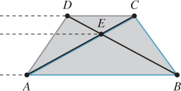
Figure 15.13: E is the centroid of square ABCD in 3D, but its projection is not the centroid of the projection of the square. This can be seen from the fact that the three dashed lines are not evenly spaced in 2D.
Fortunately, there is an efficient analog to 2D linear interpolation for projected 3D linear interpolation. This is interchangeably called hyperbolic interpolation [Bli93], perspective-correct interpolation [OG97], and rational linear interpolation [Hec90].
The perspective-correct interpolation method is simple. We can express it intuitively as, for each scalar vertex attribute u, linearly interpolate both u′ = u/z and 1/z in screen space. At each pixel, recover the 3D linearly interpolated attribute value from these by u = u′/(1/z). See the following sidebar for a more formal explanation of why this works.
 Let u(x, y, z) be some scalar attribute (e.g., albedo, u texture coordinate) that varies linearly over the polygon. Two equivalent definitions may be more intuitive: (a) u is defined at vertices by specific values and varies by barycentric interpolation between them; (b) u has the form of a 3D plane equation, u(x, y, z) = ax + by + cz + d.
When the polygon is projected into screen space by the transformation (x, y, z) → (–x/z, –y/z, –1) for an image plane at z = –1, then the function –u(x, y, z)/z varies linearly in screen space. Instead of linear interpolation in screen space, we need to perform a kind of “hyperbolic interpolation” to correctly evaluate u as follows.
Let P and Q be points on the 3D polygon, and let u(P) and u(Q) be some function that varies linearly across the plane of the 3D polygon evaluated at those points. Let P′ = –P/zP be the projection of P and Q′ = –Q/zQ be the projection of Q. At point M on line PQ that projects to M′ = αP′ + (1 – α)Q′, the value of u(M) satisfies
)
while –1/zM satisfies
)
Solving for u(M) yields
)
Because for each screen raster (i.e., row of pixels) we hold P and Q constant and vary α linearly, we can simplify the expression above to define a directly parameterized function u′ (α):
)
This is often more casually, but memorably, phrased as “In screen space, the perspective-correct interpolation of u is the quotient of the linear interpolation of u/z by the linear interpolation of 1/z.”
We can apply the perspective-correct interpolation strategy to any number of per-vertex attributes, including the vertex normals and texture coordinates. That leaves us with input data for our shade function, which remains unchanged from its implementation in the ray tracer.
15.6.4.3. 2D Barycentric Weights
To implement the perspective-correct interpolation strategy, we need only find an expression for the 2D barycentric weights at the center of each pixel. Consider the barycentric weight corresponding to vertex A of a point Q within a triangle ABC. Recall from Section 7.9 that this weight is the ratio of the distance from Q to the line containing BC to the distance from A to the line containing BC, that is, it is the relative distance across the triangle from the opposite edge. Listing 15.25 gives code for computing a barycentric weight in 2D.
Listing 15.25: Computing one barycentric weight in 2D.
1/** Returns the distance from Q to the line containing B and A. */2floatlineDistance2D(constPoint2& A,constPoint2& B,constPoint2& Q) { 3// Construct the line align:4constVector2n(A.y - B.y, B.x - A.x); 5const floatd = A.x * B.y - B.x * A.y; 6return(n.dot(Q) + d) / n.length(); 7 } 8 9/** Returns the barycentric weight corresponding to vertex A of Q in triangle ABC */10floatbary2D(constPoint2& A,constPoint2& B,constPoint2& C,constPoint2& Q) { 11returnlineDistance2D(B, C, Q) / lineDistance2D(B, C, A); 12 }
The rasterizer structure now requires a few changes from our previous version. It will need the post-projection vertices of the triangle after computing the bounding box in order to perform interpolation. We could either retain them from the bounding-box computation or just compute them again when needed later. We’ll recompute the values when needed because it trades a small amount of efficiency for a simpler interface to the bounding function, which makes the code easier to write and debug. Listing 15.26 shows the bounding box-function. The rasterizer must compute versions of the vertex attributes, which in our case are just the vertex normals, that are scaled by the  value (which we call w) for the corresponding post-projective vertex. Both of those are per-triangle changes to the code. Finally, the inner loop must compute visibility from the 2D barycentric coordinates instead of from a ray cast. The actual shading computation remains unchanged from the original ray tracer, which is good—we’re only looking at strategies for visibility, not shading, so we’d like each to be as modular as possible. Listing 15.27 shows the loop setup of the original rasterizer updated with the bounding-box and 2D barycentric approach. Listing 15.28 shows how the inner loops change.
Listing 15.26: Bounding box for the projection of a triangle, invoked by rasterize3 to establish the pixel iteration bounds.
1voidcomputeBoundingBox(constTriangle& T,constCamera& camera, 2 constImage& image, 3 Point2 V[3],int& x0,int& y0,int& x1,int& y1) { 4 5Vector2high(image.width(), image.height()); 6Vector2low(0, 0); 7 8for(intv = 0; v < 3; ++v) { 9constPoint2& X = perspectiveProject(T.vertex(v), image.width(), 10 image.height(), camera); 11 V[v] = X; 12 high = high.max(X); 13 low = low.min(X); 14 } 15 16 x0 = (int)floor(low.x); 17 x1 = (int)ceil(high.x); 18 19 y0 = (int)floor(low.y); 20 y1 = (int)ceil(high.y); 21 }
Listing 15.27: Iteration setup for a barycentric (edge align) rasterizer.
1/** 2D barycentric evaluation w. perspective-correct attributes */2voidrasterize3(Image& image,constScene& scene, 3constCamera& camera){ 4 DepthBuffer depthBuffer(image.width(), image.height(), INFINITY); 5 6// For each triangle7for(unsigned intt = 0; t < scene.triangleArray.size(); ++t) { 8constTriangle& T = scene.triangleArray[t]; 9 10// Projected vertices11Vector2V[3]; 12intx0, y0, x1, y1; 13 computeBoundingBox(T, camera, image, V, x0, y0, x1, y1); 14 15// Vertex attributes, divided by -z16floatvertexW[3]; 17Vector3vertexNw[3]; 18Point3vertexPw[3]; 19for(intv = 0; v < 3; ++v) { 20const floatw = -1.0f / T.vertex(v).z; 21 vertexW[v] = w; 22 vertexPw[v] = T.vertex(v) * w; 23 vertexNw[v] = T.normal(v) * w; 24 } 25 26// For each pixel27for(inty = y0; y < y1; ++y) { 28for(intx = x0; x < x1; ++x) { 29// The pixel center30constPoint2 Q(x + 0.5f, y + 0.5f); 31 . . . 32 33 } 34 } 35 } 36 }
Listing 15.28: Inner loop of a barycentric (edge align) rasterizer (see Listing 15.27 for the loop setup).
1// For each pixel2for(inty = y0; y < y1; ++y) { 3for(intx = x0; x < x1; ++x) { 4// The pixel center5constPoint2 Q(x + 0.5f, y + 0.5f); 6 7// 2D Barycentric weights8const floatweight2D[3] = 9 {bary2D(V[0], V[1], V[2], Q), 10 bary2D(V[1], V[2], V[0], Q), 11 bary2D(V[2], V[0], V[1], Q)}; 12 13if((weight2D[0]>0) && (weight2D[1]>0) && (weight2D[2]>0)) { 14// Interpolate depth15floatw = 0.0f; 16for(intv = 0; v < 3; ++v) { 17 w += weight2D[v] * vertexW[v]; 18 } 19 20// Interpolate projective attributes, e.g., P’, n’21Point3Pw; 22Vector3nw; 23for(intv = 0; v < 3; ++v) { 24 Pw += weight2D[v] * vertexPw[v]; 25 nw += weight2D[v] * vertexNw[v]; 26 } 27 28// Recover interpolated 3D attributes; e.g., P’ -> P, n’ -> n29constPoint3& P = Pw / w; 30constVector3& n = nw / w; 31 32const floatdepth = P.length(); 33// We could also use depth = z-axis distance: depth = -P.z34 35// Depth test36if(depth < depthBuffer.get(x, y)) { 37// Shade38Radiance3L_o; 39constVector3& w_o = -P.direction(); 40 41// Make the surface normal have unit length42constVector3& unitN = n.direction(); 43 shade(scene, T, P, unitN, w_o, L_o); 44 45 depthBuffer.set(x, y, depth); 46 image.set(x, y, L_o); 47 } 48 } 49 } 50 }
To just test coverage, we don’t need the magnitude of the barycentric weights. We only need to know that they are all positive. That is, that the current sample is on the positive side of every line bounding the triangle. To perform that test, we could use the distance from a point to a line instead of the full bary2D result. For this reason, this approach to rasterization is also referred to as testing the edge aligns at each sample. Since we need the barycentric weights for interpolation anyway, it makes sense to normalize the distances where they are computed. Our first instinct is to delay that normalization at least until after we know that the pixel is going to be shaded. However, even for performance, that is unnecessary—if we’re going to optimize the inner loop, a much more significant optimization is available to us.
In general, barycentric weights vary linearly along any line through a triangle. The barycentric weight expressions are therefore linear in the loop variables x and y. You can see this by expanding bary2D in terms of the variables inside lineDistance2D, both from Listing 15.25. This becomes
)
)
where the constants r, s, and t depend only on the triangle, and so are invariant across the triangle. We are particularly interested in properties invariant over horizontal and vertical lines, since those are our iteration directions.
For instance, y is invariant over the innermost loop along a scanline. Because the expressions inside the inner loop are constant in y (and all properties of T) and linear in x, we can compute them incrementally by accumulating derivatives with respect to x. That means that we can reduce all the computation inside the innermost loop and before the branch to three additions. Following the same argument for y, we can also reduce the computation that moves between rows to three additions. The only unavoidable operations are that for each sample that enters the branch for shading, we must perform three multiplications per scalar attribute; and we must perform a single division to compute z = –1/w, which is amortized over all attributes.
15.6.4.4. Precision for Incremental Interpolation
 We need to think carefully about precision when incrementally accumulating derivatives rather than explicitly performing linear interpolation by the barycentric coordinates. To ensure that rasterization produces complementary pixel coverage for adjacent triangles with shared vertices (“watertight rasterization”), we must ensure that both triangles accumulate the same barycentric values at the shared edge as they iterate across their different bounding boxes. This means that we need an exact representation of the barycentric derivative. To accomplish this, we must first round vertices to some imposed precision (say, one-quarter of a pixel width), and must then choose a representation and maximum screen size that provide exact storage.
The fundamental operation in the rasterizer is a 2D dot product to determine the side of the line on which a point lies. So we care about the precision of a multiplication and an addition. If our screen resolution is w × h and we want k × k subpixel positions for snapping or antialiasing, then we need ⌈log2(k·max(w, h))⌉ bits to store each scalar value. At 1920 × 1080 (i.e., effectively 2048 × 2048) with 4 × 4 subpixel precision, that’s 14 bits. To store the product, we need twice as many bits. In our example, that’s 28 bits. This is too large for the 23-bit mantissa portion of the IEEE 754 32-bit floating-point format, which means that we cannot implement the rasterizer using the single-precision float data type. We can use a 32-bit integer, representing a 24.4 fixed-point value. In fact, within that integer’s space limitations we can increase screen resolution to 8192 × 8192 at 4 × 4 subpixel resolution. This is actually a fairly low-resolution subpixel grid, however. In contrast, DirectX 11 mandates eight bits of subpixel precision in each dimension. That is because under low subpixel precision, the aliasing pattern of a diagonal edge moving slowly across the screen appears to jump in discrete steps rather than evolve slowly with motion.
15.6.5. Rasterizing Shadows
Although we are now rasterizing primary visibility, our shade routine still determines the locations of shadows by casting rays. Shadowing from a local point source is equivalent to “visibility” from the perspective of that source. So we can apply rasterization to that visibility problem as well.
A shadow map [Wil78] is an auxiliary depth buffer rendered from a camera placed at the light’s location. This contains the same distance information as obtained by casting rays from the light to selected points in the scene. The shadow map can be rendered in one pass over the scene geometry before the camera’s view is rendered. Figure 15.14 shows a visualization of a shadow map, which is a common debugging aid.
)
Figure 15.14: Left: A shadow map visualized with black = near the light and white = far from the light. Right: The camera’s view of the scene with shadows.
When a shadowing computation arises during rendering from the camera’s view, the renderer uses the shadow map to resolve it. For a rendered point to be unshadowed, it must be simultaneously visible to both the light and the camera. Recall that we are assuming a pinhole camera and a point light source, so the paths from the point to each are defined by line segments of known length and orientation. Projecting the 3D point into the image space of the shadow map gives a 2D point. At that 2D point (or, more precisely, at a nearby one determined by rounding to the sampling grid for the shadow map) we previously stored the distance from the light to the first scene point, that is, the key information about the line segment. If that stored distance is equal to the distance from the 3D point to the 3D light source, then there must not have been any occluding surface and our point is lit. If the distance is less, then the point is in shadow because the light observes some other, shadow-casting, point first along the ray. This depth test must of course be conservative and approximate; we know there will be aliasing from both 2D discretization of the shadow map and its limited precision at each point.
Although we motivated shadow maps in the context of rasterization, they may be generated by or used to compute shadowing with both rasterization and ray casting renderers. There are often reasons to prefer to use the same visibility strategy throughout an application (e.g., the presence of efficient rasterization hardware), but there is no algorithmic constraint that we must do so.
When using a shadow map with triangle rasterization, we can amortize the cost of perspective projection into the shadow map over the triangle by performing most of the computational work at the vertices and then interpolating the results. The result must be interpolated in a perspective-correct fashion, of course. The key is that we want to be perspective-correct with respect to the matrix that maps points in world space to the shadow map, not to the viewport.
Recall the perspective-correct interpolation that we used for positions and texture coordinates (see previous sidebar, which essentially relied on linearly interpolating quantities of the form  /z and w = –1/z). If we multiply world-space vertices by the matrix that transforms them into 2D shadow map coordinates but do not perform the homogeneous division, then we have a value that varies linearly in the homogeneous clip space of the virtual camera at the light that produces the shadow map. In other words, we project each vertex into both the viewing camera’s and the light camera’s homogeneous clip space. We next perform the homogeneous division for the visible camera only and interpolate the four-component homogeneous vector representing the shadow map coordinate in a perspective-correct fashion in screen space. We next perform the perspective division for the shadow map coordinate at each pixel, paying only for the division and not the matrix product at each pixel. This allows us to transform to the light’s projective view volume once per vertex and then interpolate those coordinates using the infrastructure already built for interpolating other elements. The reuse of a general interpolation mechanism and optimization of reducing transformations should naturally suggest that this approach is a good one for a hardware implementation of the graphics pipeline. Chapter 38 discusses how some of these ideas manifest in a particular graphics processor.
15.6.6. Beyond the Bounding Box
A triangle touching Ο(n) pixels may have a bounding box containing Ο(n2) pixels. For triangles with all short edges, especially those with an area of about one pixel, rasterizing by iterating through all pixels in the bounding box is very efficient. Furthermore, the rasterization workload is very predictable for meshes of such triangles, since the number of tests to perform is immediately evident from the box bounds, and rectangular iteration is generally easier than triangular iteration.
For triangles with some large edges, iterating over the bounding box is a poor strategy because n2 ≫ n for large n. In this case, other strategies can be more efficient. We now describe some of these briefly. Although we will not explore these strategies further, they make great projects for learning about hardware-aware algorithms and primary visibility computation.
15.6.6.1. Hierarchical Rasterization
Since the bounding-box rasterizer is efficient for small triangles and is easy to implement, a natural algorithmic approach is to recursively apply the bounding-box algorithm at increasingly fine resolution. This strategy is called hierarchical rasterization [Gre96].
Begin by dividing the entire image along a very coarse grid, such as into 16 × 16 macro-pixels that cover the entire screen. Apply a conservative variation of the bounding-box algorithm to these. Then subdivide the coarse grid and recursively apply the rasterization algorithm within all of the macro cells that overlapped the bounding box.
The algorithm could recur until the macro-pixels were actually a single pixel. However, at some point, we are able to perform a large number of tests either with Single Instruction Multiple Data (SIMD) operations or by using bitmasks packed into integers, so it may not always be a good idea to choose a single pixel as the base case. This is similar to the argument that you shouldn’t quicksort all the way down to a length 1 array; for small problem sizes, the constant factors affect the performance more than the asymptotic bound.
For a given precision, one can precompute all the possible ways that a line passes through a tile of samples. These can be stored as bitmasks and indexed by the line’s intercept points with the tile [FFR83, SW83]. For each line, using one bit to encode whether the sample is in the positive half-plane of the line allows an 8 × 8 pattern to fit in a single unsigned 64-bit integer. The bitwise AND of the patterns for the three line aligns defining the triangle gives the coverage mask for all 64 samples. One can use this trick to cull whole tiles efficiently, as well as avoiding per-sample visibility tests. (Kautz et al. [KLA04] extended this to a clever algorithm for rasterizing triangles onto hemispheres, which occurs frequently when sampling indirect illumination.) Furthermore, one can process multiple tiles simultaneously on a parallel processor. This is similar to the way that many GPUs rasterize today.
15.6.6.2. Chunking/Tiling Rasterization
A chunking rasterizer, a.k.a. a tiling rasterizer, subdivides the image into rectangular tiles, as if performing the first iteration of hierarchical rasterization. Instead of rasterizing a single triangle and performing recursive subdivision of the image, it takes all triangles in the scene and bins them according to which tiles they touch. A single triangle may appear in multiple bins.
The tiling rasterizer then uses some other method to rasterize within each tile. One good choice is to make the tiles 8 × 8 or some other size at which brute-force SIMD rasterization by a lookup table is feasible.
Working with small areas of the screen is a way to combine some of the best aspects of rasterization and ray casting. It maintains both triangle list and buffer memory coherence. It also allows triangle-level sorting so that visibility can be performed analytically instead of using a depth buffer. That allows both more efficient visibility algorithms and the opportunity to handle translucent surfaces in more sophisticated ways.
15.6.6.3. Incremental Scanline Rasterization
For each row of pixels within the bounding box, there is some location that begins the span of pixels covered by the triangle and some location that ends the span. The bounding box contains the triangle vertically and triangles are convex, so there is exactly one span per row (although if the span is small, it may not actually cover the center of any pixels).
A scanline rasterizer divides the triangle into two triangles that meet at a horizontal line through the vertex with the median vertical ordinate of the original triangle (see Figure 15.15). One of these triangles may have zero area, since the original triangle may contain a horizontal edge.
)
Figure 15.15: Dividing a triangle horizontally at its middle vertex.
The scanline rasterizer computes the rational slopes of the left and right edges of the top triangle. It then iterates down these in parallel (see Figure 15.16). Since these edges bound the beginning and end of the span across each scan-line, no explicit per-pixel sample tests are needed: Every pixel center between the left and right edges at a given scanline is covered by the triangle. The rasterizer then iterates up the bottom triangle from the bottom vertex in the same fashion. Alternatively, it can iterate down the edges of the bottom triangle toward that vertex.
)
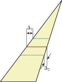
Figure 15.16: Each span’s starting point shifts Δ1 from that of the previous span, and its ending point shifts Δ2.
The process of iterating along an edge is performed by a variant of either the Digital Difference Analyzer (DDA) or Bresenham line algorithm [Bre65], for which there are efficient floating-point and fixed-point implementations.
Pineda [Pin88] discusses several methods for altering the iteration pattern to maximize memory coherence. On current processor architectures this approach is generally eschewed in favor of tiled rasterization because it is hard to schedule for coherent parallel execution and frequently yields poor cache behavior.
15.6.6.4. Micropolygon Rasterization
Hierarchical rasterization recursively subdivided the image so that the triangle was always small relative to the number of macro-pixels in the image. An alternative is to maintain constant pixel size and instead subdivide the triangle. For example, each triangle can be divided into four similar triangles (see Figure 15.17). This is the rasterization strategy of the Reyes system [CCC87] used in one of the most popular film renderers, RenderMan. The subdivision process continues until the triangles cover about one pixel each. These triangles are called micropolygons. In addition to triangles, the algorithm is often applied to bilinear patches, that is, Bézier surfaces described by four control points (see Chapter 23).
)
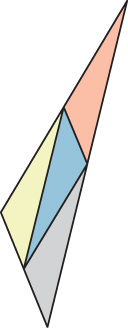
Figure 15.17: A triangle subdivided into four similar triangles.
Subdividing the geometry offers several advantages over subdividing the image. It allows additional geometric processing, such as displacement mapping, to be applied to the vertices after subdivision. This ensures that displacement is performed at (or slightly higher than) image resolution, effectively producing perfect level of detail. Shading can be performed at vertices of the micropolygons and interpolated to pixel centers. This means that the shading is “attached” to object-space locations instead of screen-space locations. This can cause shading features, such as highlights and edges, which move as the surface animates, to move more smoothly and with less aliasing than they do when we use screen-space shading. Finally, effects like motion blur and defocus can be applied by deforming the final shaded geometry before rasterization. This allows computation of shading at a rate proportional to visible geometric complexity but independent of temporal and lens sampling.