Factorial Analysis
One of the reasons that the development of the analysis of variance represents such a major step forward in the science of data analysis is that it provides the ability to study the simultaneous effects of two or more factors on the outcome variable. Prior to the groundwork that Fisher did with ANOVA, researchers were limited to studying one variable at a time, usually just two levels of that factor at a time.
This situation meant that researchers could not investigate the joint effect of two or more factors. For example, it may be that men have a different attitude toward a politician when they are over 50 years of age than they do earlier in their lives. Furthermore, it may be that women’s attitude toward that politician do not change as a function of their age. If we had to study the effects of sex and age separately, we wouldn’t be able to determine that a joint effect—termed an interaction in statistical jargon—exists.
But we can accommodate more than just one factor in an ANOVA—or, of course, in a regression analysis. When you simultaneously analyze how two or more factors are related to an outcome variable, you’re said to be using factorial analysis.
And when you can study and analyze the effects of more than just one variable at a time, you get more bang for your buck. The costs of running an experiment are often just trivially greater when you study additional variables than when you study only one.
It also happens that adding one or more factors to a single factor ANOVA can increase its statistical power. In a single-factor ANOVA, variation in the outcome variable that can’t be attributed to the factor gets tossed into the mean square residual. It can happen that such variation might be associated with another factor (or, as you’ll see in the next chapter, a covariate). Then that variation could be removed from the mean square error—which, when decreased, increases the value of F-ratios in the analysis, thus increasing the tests’ statistical power.
Excel’s Data Analysis add-in includes a tool that accommodates two factors at once, but it has drawbacks. In addition to a problem I’ve noted before, that the results do not come back as formulas but as static values, the ANOVA: Two-Factor with Replication tool requires that you arrange your data in a highly idiosyncratic fashion, and it cannot accommodate unequal group sizes, nor can it accommodate more than two factors. Covariates are out.
If you use regression instead, you don’t have to live with those limits. To give you a basis for comparison, let’s look at the results of the ANOVA: Two-Factor with Replication tool.
The ANOVA tool used in Figure 7.16 is helpful in that it returns the average and variance of the outcome variable, as well as the count, for each group in the design. My own preference would be to use a pivot table to report these descriptive statistics, because that’s a live analysis and the table returned by the ANOVA tool is, again, static values. With a pivot table I can add, delete, or edit observations and have the pivot table update itself. With static values I have to run the ANOVA tool over again.
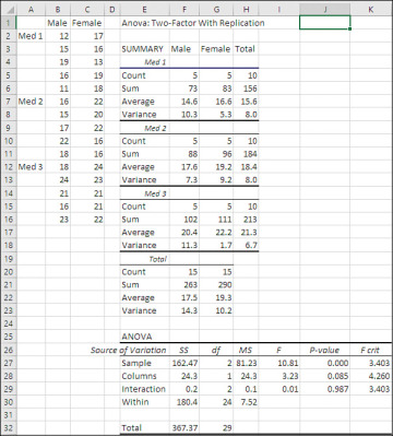
Figure 7.16 The ANOVA: Two-Factor with Replication tool will not run if different groups have different numbers of observations.
The ANOVA table at the end of the results shows a couple of features that don’t appear in the Data Analysis add-in’s Single Factor version. Notice that rows 27 and 28 show a Sample and a Column source of variation. The Column source of variation refers to sex: Values for males are in column B and values for females are in column C. The Sample data source refers to whatever variable has values that occupy different rows. In Figure 7.16, values for Med 1 are in rows 2 through 6, Med 2 in rows 7 through 11, and Med 3 in rows 12 through 16.
You’ll want to draw your own conclusions regarding the convenience of the data layout (required, by the way, by the Data Analysis tool) and regarding the labeling of the factors in the ANOVA table.
The main point is that both factors, Sex (labeled Columns in cell E28) and Medication (labeled Sample in cell E27), exist as sources of variation in the ANOVA table. Males’ averages differ from females’ averages, and that constitutes a source of variation. The three kinds of medication also differ from one another’s averages—another source of variation.
There is also a third source labeled Interaction, which refers to the joint effect of the Sex and Medication variables. At the interaction level, groups are considered to constitute combinations of levels of the main factors: For example, Males who get Med 2 constitute a group, as do Females who get Med 1. Differences due to the combined main effects—not just Male compared to Female, or Med 1 compared to Med 3—are collectively referred to as the interaction between, here, Sex and Treatment.
The ANOVA shown in Figure 7.16 evaluates the effect of Sex as not significant at the .05 level (see cell J28, which reports the probability of an F-ratio of 3.23 with 1 and 24 degrees of freedom as 8.5% when there is no difference in the populations). Similarly, there is no significant difference due to the interaction of Sex with Treatment. Differences between the means of the six design cells (two sexes times three treatments) are not great enough to reject the null hypothesis of no differences among the six groups. Only the Treatment main effect is statistically significant. If, from the outset, you intended to use planned orthogonal contrasts to test the differences between specific means, you could do so now and enjoy the statistical power available to you. In the absence of such planning, you could use the Scheffé procedure, hoping that you wouldn’t lose too much statistical power as a penalty for having failed to plan your contrasts.
Factorial Analysis with Orthogonal Coding
However, there’s no reason that you couldn’t use orthogonal coefficients in the vectors. You wouldn’t do so on a post hoc basis to increase statistical power, because that requires you to choose your comparisons before seeing the results. However, with equal group sizes you could still use orthogonal codes in the vectors to make some of the computations more convenient. Figure 7.17 shows the data from Figure 7.16 laid out as a list, with vectors that represent the Sex and the Treatment variables.
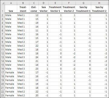
Figure 7.17 The two-factor problem from Figure 7.16 laid out for regression analysis.
The data set in Figure 7.17 has one vector in column D to represent the Sex variable. Because that factor has only two levels, one vector is sufficient to represent it. The data set also has two vectors in columns E and F to represent the Treatment factor. That factor has three levels, so two vectors are needed. Finally, two vectors representing the interaction between Sex and Treatment occupy columns G and H.
The interaction vectors are easily populated by multiplying the main effect vectors. The vector in column G is the result of multiplying the Sex vector by the Treatment 1 vector. The vector in column H results from the product of the Sex vector and the Treatment 2 vector.
The choice of codes in the Sex and Treatment vectors is made so that all the vectors will be mutually orthogonal. That’s a different reason from the one used in Figure 7.15, where the idea is to specify contrasts that are of particular theoretical interest—the means of particular groups, and the combinations of group means, that you hope will inform you about the way that independent variables work together and with the dependent variable to bring about the observed outcomes.
But in Figure 7.17, the codes are chosen simply to make the vectors mutually orthogonal because it makes the subsequent analysis easier. The most straightforward way to do this is as follows.
1. Supply the first vector with codes that will contrast the first level of the factor with the second level, and ignore other levels. In Figure 7.17, the first factor has only two levels, so it requires only one vector, and the two levels exhaust the factor’s information. Therefore, give one level of Sex a code of 1 and the other level a code of −1.
2. Do the same for the first level of the second factor. In this case the second factor is Treatment, which has three levels and therefore two vectors. The first level, Med 1, gets a 1 in the first vector and the second level, Med 2, gets a −1. All other levels, in this case Med 3, get 0’s. This conforms to what was done with the Sex vector in Step 1.
3. In the second (and subsequent) vectors for a given factor, enter codes that contrast the first two levels with the third level (or the first three with the fourth, or the first four with the fifth, and so on). That’s done in the second Treatment variable by assigning the code 1 to both Med 1 and Med 2, and −2 to Med 3. This contrasts the first two levels from the third. If there were other levels shown in this vector they would be assigned 0’s.
The interaction vectors are obtained by multiplication of the main effect vectors, as described in the preceding steps. Now, Figure 7.18 shows the analysis of this data set.
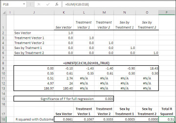
Figure 7.18 The orthogonal vectors all correlate 0.0 with one another.
In Figure 7.18, the correlation matrix in the range K2:O6 shows that the correlations between each pair of vectors is 0.0.
The fact that all the correlations between the vectors are 0.0 means that the vectors share no variance. Because they share no variance, it’s impossible for the relationships of two vectors with the outcome variable to overlap. Any variance shared by the outcome variable and, say, the first Treatment vector is unique to that Treatment vector. When all the vectors are mutually orthogonal, there is no ambiguity about where to assign variance shared with the outcome variable.
In the range J9:O13 of Figure 7.18 you’ll find the results returned by LINEST() for the data shown in Figure 7.17. Not that it matters for present purposes, but the statistical significance of the overall regression is shown in cell M15, again using the F.DIST.RT() function. More pertinent is that the R2 for the regression, 0.51, is found in cell J11.
The range K18:O18 contains the R2 values for each coded vector with the outcome variable. Excel provides a function, RSQ(), that returns the square of the correlation between two variables. So the formula in cell K18 is:
=RSQ($C$2:$C$31,D2:D31)
Cell P18 shows the sum of the five R2 values. That sum, 0.51, is identical to the R2 for the full regression equation that’s returned by LINEST() in cell J11. We have now partitioned the R2 for the full equation into five constituents.
Figure 7.19 ties the results of the regression analysis back to the two-factor ANOVA in Figure 7.16.
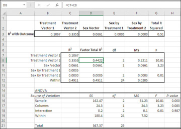
Figure 7.19 Compare the result of using sums of squares with the using proportions of variance.
In Figure 7.19 I have brought forward the R2 values for the coded vectors, and the total regression R2, from the range K18:P18 in Figure 7.18. Recall that these R2 values are actually measures of the proportion of total variance in the outcome variable associated with each vector. So the total amount of variance explained by the coded vectors is 51%, and therefore 49% of the total variance remains unexplained. That 49% of the variance is represented by the mean square residual (or mean square within, or mean square error) component—the divisor for the F-ratios.
The three main points to take from Figure 7.19 are discussed next.
Unique Proportions of Variance
The individual R2 values for each vector can simply be summed to get the R2 for the total regression equation. The simple sum is accurate because the vectors are mutually orthogonal. Each vector accounts for a unique proportion of the variance in the outcome. Therefore there is no double-counting of the variance, as there would be if the vectors were correlated. The total of the individual R2 values equals the total R2 for the full regression.
Proportions of Variance Equivalent to Sums of Squares
Compare the F-ratios from the analysis in the range C7:G12, derived from proportions of variance, with the F-ratios from the ANOVA in B15:H21, derived from the sums of squares. The F-ratios are identical, and the conclusions that you would draw from each analysis: that the sole significant difference is due to the treatments, and no difference emerges as a function of either sex or the interaction of sex with treatment.
The proportions of variance bear the same relationships to one another as do the sums of squares. That’s not surprising. It’s virtually by definition, because each proportion of variance is simply the sum of squares for that component divided by the total sum of squares—a constant. All the proportions of variance, including that associated with mean square residual, total to 1.0, so if you multiply an individual proportion of variance such as 0.4422 in cell D8, by the total sum of squares (367.37 in cell D21), you wind up with the sum of squares for that component (162.47 in cell D16). Generally, proportions of variance speak for themselves, while sums of squares don’t. If you say that 44.22% of the variance in the outcome variable is due to the treatments, I immediately know how important the treatments are. If you say that the sum of squares due to treatments is 162.47, I suggest that you’re not communicating with me.
Summing Component Effects
The traditional ANOVA shown in B15:H21 of Figure 7.19 does not provide inferential information for each comparison. The sums of squares, the mean squares and the F-ratios are for the full factor. Traditional methods cannot distinguish, for example, the effect of Med 1 versus Med 2 from the effect of Med 2 versus Med 3. That’s what multiple comparisons are for.
However, we can get an R2 for each vector in the regression analysis. For example, the R2 values in cells C7 and C8 are 0.1067 and 0.3355. Those proportions of variance are attributable to whatever comparison is implied by the codes in their respective vectors. As coded in Figure 7.17, Treatment Vector 1 compares Med 1 with Med 2, and Treatment Vector 2 compares the average of Med 1 and Med 2 with Med 3. Notice that if you add the two proportions of variance together and multiply by the total sum of squares, 367.37, you get the sum of squares associated with the Treatment factor in cell D16, returned by the traditional ANOVA.
The individual vectors can be tested in the same way as the collective vectors (one for each main effect and one for the interaction). Figure 7.20 demonstrates that more fine-grained analysis.
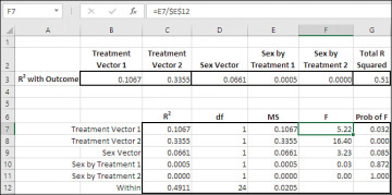
Figure 7.20 The question of what is being tested by a vector’s F-ratio depends on how you have coded the vector.
The probabilities in the range G7:G11 of Figure 7.20 indicate the likelihoods of obtaining an F-ratio as large as those in F7:F11 if the differences in means that are defined by the vectors’ codes were all 0.0 in the population. So, if you had specified an alpha of 0.05, you could reject the null hypothesis for the Treatment 1 vector (Med 1 versus Med 2) and the Treatment 2 vector (the average of Med 1 and Med 2 versus Med 3). But if you had selected an alpha of 0.01, you could reject the null hypothesis for only the comparison in Treatment Vector 2.
Factorial Analysis with Effect Coding
Chapter 3, in the section titled “Partial and Semipartial Correlations,” discussed how the effect of a third variable can be statistically removed from the correlation between two other variables. The third variable’s effect can be removed from both of the other two variables (partial correlation) or from just one of the other two (semipartial correlation). We’ll make use of semipartial correlations—actually, the squares of the semipartial correlations—in this section. The technique also finds broad applicability in situations that involve unequal numbers of observations per group.
Figure 7.21 shows how the orthogonal coding from Figure 7.17, used in Figures 7.18 through 7.20, has been changed to effect coding.
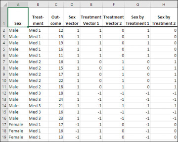
Figure 7.21 As you’ll see, effect coding results in vectors that are not wholly orthogonal.
In the Sex vector, Males are assigned 1’s and Females are assigned −1’s. With a two-level factor such as Sex, orthogonal coding is identical to effect coding.
The first Treatment vector assigns 1’s to Med 1, 0’s to Med 2, and −1’s to Med 3. So Treatment Vector 1 contrasts Med 1 with Med 3. Treatment Vector 2 assigns 0’s to Med 1, 1’s to Med 2 and (again) −1’s to Med 3, resulting in a contrast of Med 2 with Med 3. Thus, although they both provide tests of the Treatment variable, the two Treatment vectors define different contrasts than are defined by the orthogonal coding used in Figure 7.17.
Figure 7.22 displays the results of effect coding on the outcome variable, which has the same values as in Figure 7.17.
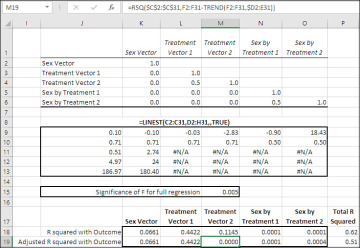
Figure 7.22 Vectors that represent different levels of a given factor are correlated if you use effect coding.
Notice that not all the off-diagonal entries in the correlation matrix, in the range K2:O6, are 0.0. Treatment Vector 1 has a 0.50 correlation with Treatment Vector 2, and the two vectors that represent the Sex by Treatment interaction also correlate at 0.50. This is typical of effect coding, although it becomes evident in the correlation matrix only when a main effect has at least three levels (as does Treatment in this example).
The result is that the vectors are not all mutually orthogonal, and therefore we cannot simply add up each variable’s R2 to get the R2 for the full regression equation, as is done in Figures 7.18 through 7.20. Furthermore, because the R2 of the vectors do not represent unique proportions of variance, we can’t simply use those R2 values to test the statistical significance of each vector.
Instead, it’s necessary to use squared semipartial correlations to adjust the R2 values so that they are orthogonal, representing unique proportions of the variance of the outcome variable.
In Figure 7.22, the LINEST() analysis in the range J9:O13 returns the same values as the LINEST() analysis with orthogonal coding in Figure 7.18, except for the regression coefficients, the constant, and their standard errors. In other words, the differences between orthogonal and effect coding make no difference to the equation’s R2, its standard error of estimate, the F-ratio, the degrees of freedom for the residual, or the regression and residual sums of squares. This is not limited to effect and orthogonal coding. Regardless of the method you apply—dummy coding, for example—it makes no difference to the statistics that pertain to the equation generally. The differences in coding methods show up when you start to look at variable-to-variable quantities, such as a vector’s regression coefficient or its simple R2 with the outcome variable.
Notice the table of R2 values in rows 18 and 19 of Figure 7.22. The R2 values in row 18 are raw, unadjusted proportions of variance. They do not represent unique proportions shared with the outcome variable. As evidence of that, the totals of the R2 values in rows 18 and 19 are shown in cells P18 and P19. The value in cell P18, the total of the unadjusted R2 values in row 18, is 0.62, well in excess of the R2 for the full regression reported by LINEST() in cell J11.
Most of the R2 values in row 19, by contrast, are actually squared semipartial correlations. Two that should catch your eye are those in L19 and M19. Because the two vectors for the Treatment variable are correlated, the proportions of variance attributed to them in row 18 via the unadjusted R2 values double-count some of the variance shared with the outcome variable. It’s that double-counting that inflates the total of the R2 values to 0.62 from its legitimate value of 0.51.
What we want to do is remove the effect of the vectors to the left of the second Treatment vector from the second Treatment vector itself. You can see how that’s done most easily by starting with the R2 in cell K19, and then following the trail of bread crumbs through cells L19 and M19, as follows:
Cell K19: The formula is as follows:
=RSQ($C$2:$C$31,D2:D31).
The vector in column D, Sex, is the leftmost variable in LINEST()’s X-value arguments. (Space limits prevent the display of column D in Figure 7.22, but it’s visible in Figure 7.21 and, of course, in the downloaded workbook for Chapter 7.) No variables precede the vector in column D and so there’s nothing to partial out of the Sex vector: We just accept the raw R2.
Cell L19: The formula is:
=RSQ($C$2:$C$31,E2:E31-TREND(E2:E31,$D2:D31))
The fragment TREND(E2:E31,$D2:D31) predicts the values in E2:E31 (the first Treatment vector) from the values in the Sex vector (D2:D31). You can see from the correlation matrix at the top of Figure 7.22 that the correlation between the Sex vector and the first Treatment vector is 0.0. In that case, the regression of Treatment 1 on Sex predicts the mean of the Treatment 1 vector. The vector has equal numbers of 1’s, 0’s and −1’s, so its mean is 0.0. In short, the R2 formula subtracts 0.0 from the codes in E2:E31 and we wind up with the same result in L19 as we do in L18.
Cell M19: The formula is:
=RSQ($C$2:$C$31,F2:F31-TREND(F2:F31,$D2:E31))
Here’s where the squared semipartial kicks in. This fragment:
TREND(F2:F31,$D2:E31)
predicts the values for the second Treatment vector, F2:F31, based on its relationship to the vectors in column D and column E, via the TREND() function. When those predicted values are subtracted from the actual codes in column F, via this fragment:
F2:F31-TREND(F2:F31,$D2:E31)
you’re left with residuals: the values for the second Treatment vector in F2:F31 that have their relationship with the Sex and the first Treatment vector removed. With those effects gone, what’s left of the codes in F2:F31 is unique and unshared with either Sex or Treatment Vector 1. As it happens, the result of removing the effects of the Sex and the Treatment 1 vectors eliminates the original relationship between the Treatment 2 vector and the outcome variable, leaving both a correlation and an R2 of 0.0. The double-counting of the shared variance is also eliminated and, when the adjusting formulas are extended through O19, the sum of the proportions of variance in K19:O19 equals the R2 for the full equation in cell J11.
The structure of the formulas that calculate the squared semipartial correlations deserves a little attention because it can save you time and headaches. Here again is the formula used in cell L19:
=RSQ($C$2:$C$31,E2:E31-TREND(E2:E31,$D2:D31))
The address $C$2:$C$31 contains the outcome variable. It is a fixed reference (although it might as well be treated as a mixed reference, $C2:$C31, because we won’t intentionally paste it outside row 19). As we copy and paste it to the right of column L, we want to continue to point the RSQ function at C2:C31, and anchoring the reference to column C accomplishes that.
The other point to note in the RSQ() formula is the mixed reference $D2:D31. Here’s what the formula changes to as you copy and paste it, or drag and drop it, from L19 one column right into M19:
=RSQ($C$2:$C$31,F2:F31-TREND(F2:F31,$D2:E31))
Notice first that the references to E2:E31 in L19 have changed to F2:F31, in response to copying the formula one column right. We’re now looking at the squared semipartial correlation between the outcome variable in column C and the second Treatment vector in column F.
But the TREND() fragment shows that we’re adjusting the codes in F2:F31 for their relationship to the codes in columns D and E. By dragging the formula on column to the right:
$C$2:$C$31 remains unchanged. That’s where the outcome variable is located.
E2:E31 changes to F2:F31. That’s the address of the second Treatment vector.
$D2:D31 changes to $D2:E31. That’s the address of the preceding predictor variables. We want to remove from the second Treatment vector the variance it shares with the preceding predictors: the Sex vector and the first Treatment vector.
By the time the formula reaches O19:
$C$2:$C$31 remains unchanged.
E2:E31 changes to H2:H31.
$D2:D31 changes to $D2:G31.
The techniques I’ve outlined in this section become even more important in Chapter 8, where we take up the analysis of covariance (ANCOVA). In ANCOVA you use variables that are measured on an interval or ratio scale as though they were factors measured on a nominal scale. The idea is not just to make successive R2 values unique, as discussed in the present section, but to equate different groups of subjects as though they entered the experiment on a common footing—in effect, giving random assignment an assist.

