Effect Coding
Another type of coding, called effect coding, contrasts each group mean following an ANOVA with the grand mean of all the observations.
This aspect of effect coding—contrasting group means with the grand mean rather than with a specified group, as with dummy coding—is due to the use of −1 instead of 0 as the code for the group that gets the same code throughout the coded vectors. Because the contrasts are with the grand mean, each contrast represents the effect of being in a particular group.
Coding with -1 Instead of 0
Let’s take a look at an example before getting into the particulars of effect coding. See Figure 7.9.

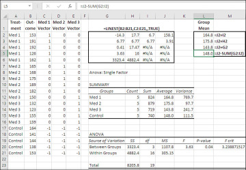
Figure 7.9 The coefficients in LINEST() equal each group’s distance from the grand mean.
Figure 7.9 has the same data set as Figure 7.6, except that the Control group has the value −1 throughout the three coded vectors, instead of 0 as in dummy coding. Some of the LINEST() results are therefore different than in Figure 7.6. The regression coefficients in Figure 7.9 differ from those in Figure 7.6, as do their standard errors. All the remaining values are the same: R2, the standard error of estimate, the F-ratio, the residual degrees of freedom, and the regression and residual sums of squares—all those remain the same, just as they do with the third method of coding that this chapter considers, planned orthogonal contrasts.
In dummy coding, the constant returned by LINEST() is the mean of the group that’s assigned 0’s throughout the coded vectors—usually a control group. In effect coding, the constant is the grand mean. The constant is easy to find. It’s the value in the first row (along with the regression coefficients) and in the rightmost column of the LINEST() results.
Because the constant equals the grand mean, it’s easy to calculate the group means from the constant and the regression coefficients. Each coefficient, as I mentioned at the start of this section, represents the difference between the associated group’s mean and the grand mean. So, to calculate the group means, add the constant to the regression coefficients. That’s been done in Figure 7.9, in the range L2:L4. The formulas used in that range are given as text in M2:M4.
Notice that the three formulas add the constant (the grand mean) to a regression coefficient (a measure of the effect of being in that group, the distance of the group mean above or below the grand mean). The fourth formula in L5 is specific to the group assigned codes of −1, and it subtracts the other coefficients from the grand mean to calculate the mean of that group.
Also notice that the results of the formulas in L2:L5 equal the group means reported in the range J12:J15 by the Data Analysis add-in’s ANOVA: Single Factor tool. It’s also worth verifying that the F-ratio, the residual degrees of freedom, and the regression and residual sums of squares equal those reported by that tool in the range H20:K21.
Relationship to the General Linear Model
The general linear model is a useful way of conceptualizing the components of a value on an outcome variable. Its name makes it sound a lot more forbidding than it really is. Here’s the general linear model in its simplest form:
Yij = μ + aj + εij
The formula uses Greek instead of Roman letters to emphasize that it’s referring to the population from which observations are sampled, but it’s equally useful to consider that it refers to a sample taken from that population:

The idea is that each observation Yij can be considered as the sum of three components:
The grand mean, μ
The effect of treatment j, aj
The quantity εij that represents the deviation of an individual score Yij from the combination of the grand mean and the jth treatment’s effect.
Here it is in the context of a worksheet (see Figure 7.10):

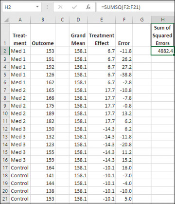
Figure 7.10 Observations broken down in terms of the components of the general linear model.
In Figure 7.10, each of the 20 observations in Figure 7.9 have been broken down into the three components of the general linear model: the grand mean in the range D2:D21, the effect of each treatment group in E2:E21, and the so-called “error” involved with each observation.
If you didn’t expect that one or more treatments would have an effect on the subjects receiving that treatment, then your best estimate of the value of a particular observation would be the grand mean (in this case, that’s 158.1).
But suppose you expected that the effect of a treatment would be to raise the observed values for the subjects receiving that treatment above, or lower them below, the grand mean. In that case your best estimate of a given observation would be the grand mean plus the effect, whether positive or negative, associated with that treatment. In the case of, say, the observation in row 5 of Figure 7.10, your expectation would be 158.1 + 6.7, or 164.8. If you give the matter a little thought, you’ll see why that figure, 164.8, must be the mean outcome score for the Med 1 group.
Although the mean of its group is your best expectation for any one of its members, most—typically all—of the members of a group will have a score on the outcome variable different from the mean of the group. Those quantities (differences, deviations, residuals, errors, or whatever you prefer to call them) are shown in the range F2:F21 as the result of subtracting the grand mean and the group’s treatment effect from the actual observation. For example, the value in cell F2 is returned by this formula:
=B2-D2-E2
The purpose of a regression equation is to minimize the sum of the squares of those errors. When that’s done, the minimized result is called the Residual Sum of Squares in the context of regression, and the Sum of Squares Within in the context of ANOVA.
Note the sum of the squared errors in cell H2. It’s returned by this formula:
=SUMSQ(F2:F21)
The SUMSQ() function squares the values in its argument and totals them. That’s the same value as you’ll find in Figure 7.9, cells H21, the Sum of Squares Within Groups from the ANOVA, and H6, the residual sum of squares from LINEST(). As Figure 7.10 shows, the sum of squares is based on the mean deviations from the grand mean, and on the individual deviations from the group means.
It’s very simple to move from dummy coding to effect coding. Rather than assigning codes of 0 throughout the coding vectors to one particular group, you assign codes of −1 to one of the groups—not necessarily a control group—throughout the vectors. If you do that in the key range used by VLOOKUP(), you need to make that replacement in only as many key range cells as you have vectors. You can see in Figure 7.9 that this has been done in the range C17:E21, which contains −1’s rather than 0’s. I assigned the −1’s to the control group not because it’s necessarily desirable to do so, but to make comparisons with the dummy coding used in Figure 7.6.
Regression analysis with a single factor and effect coding handles unequal group sizes accurately, and so does traditional ANOVA. Figure 7.11 shows an analysis of a data set with unequal group sizes.

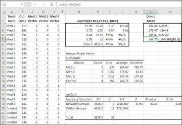
Figure 7.11 The ANOVA: Single Factor tool returns the group counts in the range H11:H14.
Notice that the regression equation returns as the regression coefficients the effect of being in each of the treatment groups. In the range L2:L5, the grand mean (which is the constant in the regression equation) is added to each of the regression coefficients to return the actual mean for each group. Compare the results with the means returned by the Data Analysis add-in in the range J11:J14.
Notice that the grand mean is the average of the group means, 158.41, rather than the mean of the individual observations, 158.6. This situation is typical of designs in which the groups have different numbers of observations.
Both the traditional ANOVA approach and the regression approach manage the situation of unequal group sizes effectively. But if you have groups with very discrepant numbers of observations and very discrepant variances, you’ll want to keep in mind the discussion from Chapter 6 regarding their combined effects on probability estimates: If your larger groups also have the larger variances, your apparent tests will tend to be conservative. If the larger groups have the smaller variances, your apparent tests will tend to be liberal.
Multiple Comparisons with Effect Coding
Dummy coding largely defines the comparisons of interest to you. The fact that you choose dummy coding as the method of populating the vectors in the data matrix implies that you want to compare one particular group mean, usually that of a control group, with the other group means in the data set. The Dunnett method of multiple comparisons is often the method of choice when you’ve used dummy coding.
A more flexible method of multiple comparisons is called the Scheffé method. It is a post hoc method, meaning that you can use it after you’ve seen the results of the overall analysis and that you need not plan ahead of time what comparisons you’ll make. The Scheffé method also enables you to make complex contrasts, such as the mean of two groups versus the mean of three other groups.
There’s a price to that flexibility, and it’s in the statistical power of the Scheffé method. The Scheffé will fail to declare comparisons as statistically significant that other methods would. That’s a problem and it’s a good reason to consider other methods such as planned orthogonal contrast (discussed later in this chapter).
To use the Scheffé method, you need to set up a matrix that defines the contrasts you want to make. See Figure 7.12.

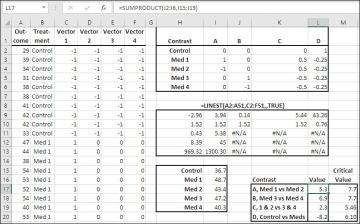
Figure 7.12 The matrix of contrasts defines how much weight each group mean is given.
Consider Contrast A, in the range I2:I6 of Figure 7.12. Cell I3 contains a 1 and cell I4 contains a −1; the remaining cells in I2:I6 contain 0’s. The values in the matrix are termed contrast coefficients. You multiply each contrast coefficient by the mean of the group it belongs to. Therefore, I2:I6 defines a contrast in which the mean of Med 2 (coefficient of −1) is subtracted from the mean of Med 1 (coefficient of 1), and the remaining group means do not enter the contrast.
Similarly, Contrast B, in J2:J6, also contains a 1 and a −1, but this time it’s the difference between Med 3 and Med 4 that’s to be tested.
More complex contrasts are possible, of course. Contrast C compares the average of Med 1 and Med 2 with the average of Med 3 and Med 4, and Contrast D compares Control with the average of the four medication groups.
A regression analysis of the effect-coded data in A2:F51 appears in H9:L13. An F-test of the full regression (which is equivalent to a test of the deviation of the R2 value in H11 from 0.0) could be managed with this formula:
=F.DIST.RT(H12,4,I12)
It returns 0.00004, and something like 4 in 100,000 replications of this experiment would return an F-ratio of 8.39 or greater if there were no differences between the population means. So you move on to a multiple comparisons procedure to try to pinpoint the differences that bring about so large an F-ratio.
You can pick up the group means by combining the constant returned by LINEST() in cell L9 (which, with effect coding, is the mean of the group means) with the individual regression coefficients. For example, the mean of the Med 1 group is returned in cell I16 with this formula:
=K9+$L$9
The formula for the mean of the group assigned −1’s throughout the coding matrix is just a little more complicated. It is the grand mean minus the sum of the remaining regression coefficients. So, the formula for the control group in cell I15 is:
=$L$9-SUM(H9:K9)
With the five group means established in the range I15:I19, you can apply the contrasts you defined in the range I2:L6 by multiplying each group mean by the associated contrast coefficient for that contrast. Excel’s SUMPRODUCT() function is convenient for that: It multiplies the corresponding elements in two arrays and returns the sum of the products. Therefore, this formula in cell L17:
=SUMPRODUCT(I2:I6,I15:I19)
has this effect:
=I2*I15 + I3*I16 + I4*I17 + I5*I18 + I6*I19
which results in the value 5.3. The formula in cell L18 moves one column to the right in the contrast matrix:
=SUMPRODUCT(J2:J6,I15:I19)
and so on through the fourth contrast.
The final step in the Scheffé method is to determine a critical value that the contrast values in L17:L20 must exceed to be regarded as statistically significant. Here’s the formula, which looks a little forbidding in Excel syntax:
=SQRT((5−1)*F.INV(0.95,4,I12))*SQRT(($I$13/$I$12)
*(J2^2/10+J3^2/10+J4^2/10+J5^2/10+J6^2/10))
Here it is using more conventional notation:

where:
k is the number of groups.
Fdf1,df2 is the value of the F distribution at the alpha level you select, such as 0.05 or 0.01. In the Excel version of the formula just given, I chose the .05 level, using 0.95 as the argument to the F.INV() function because it returns the F-ratio that has, in this case, 0.95 of the distribution to its left. I could have used, instead, F.INV.RT(0.05,4,I12) to return the same value.
MSR is the mean square residual from the LINEST() results, obtained by dividing the residual sum of squares by the degrees of freedom for the residual.
C is the contrast coefficient. Each contrast coefficient is squared and divided by nj, the number of observations in the group. The results of the divisions are summed.
The critical value varies across the contrasts that have different coefficients. To complete the process, compare the value of each contrast with its critical value. If the absolute value of the contrast exceeds the critical value, then the contrast is considered significant at the level you chose for the F value in the formula for the critical value.
In Figure 7.12, the critical values are shown in the range M17:M20. Only one contrast has an absolute value that exceeds its associated critical value: Contrast D, which contrasts the mean of the Control group with the average of the means of the four remaining groups.
I mentioned at the start of this section that the Scheffé method is at once the least statistically powerful and the most flexible of the multiple comparison methods. You might want to compare the results reported here with the results of planned orthogonal contrasts, discussed in the next section. Planned orthogonal contrasts are at once the most statistically powerful and the least flexible of the multiple comparison methods. When we get to the multiple comparisons in the next section, you’ll see that the same data set returns very different outcomes.

