- 5.1 Frequency-Flat Wireless Channels
- 5.2 Equalization of Frequency-Selective Channels
- 5.3 Estimating Frequency-Selective Channels
- 5.4 Carrier Frequency Offset Correction in Frequency-Selective Channels
- 5.5 Introduction to Wireless Propagation
- 5.6 Large-Scale Channel Models
- 5.7 Small-Scale Fading Selectivity
- 5.8 Small-Scale Channel Models
- 5.9 Summary
- Problems
This chapter is from the book
This chapter is from the book
This chapter is from the book
5.2 Equalization of Frequency-Selective Channels
In this and subsequent sections, we generalize the development in Section 5.1 to frequency-selective fading channels. We focus specifically on equalization, assuming that channel estimation, frame synchronization, and frequency offset synchronization have been performed. We solve the channel estimation problem in Section 5.3 and the frame and frequency offset synchronization problems in Section 5.4. First we develop the discrete-time received signal model, including a frequency-selective channel and AWGN. Then we develop three approaches for linear equalization. The first approach is based on constructing an FIR filter that approximately inverts the effective channel. The second approach is to insert a special prefix in the transmitted signal to permit frequency-domain equalization at the receiver, in what is called SC-FDE. The third approach also uses a cyclic prefix but precodes the information in the frequency domain, in what is called OFDM modulation. As the equalization removes intersymbol interference, standard symbol detection follows the equalization operations.
5.2.1 Discrete-Time Model for Frequency-Selective Fading
In this section, we develop a received signal model for general frequency-selective channels, generalizing the results for a single path in Section 5.1.1. Assuming perfect synchronization, the received complex baseband signal after matched filtering but prior to sampling is
Essentially, y(t) takes the form of a complex pulse-amplitude modulated signal but where g(t) is replaced by  . Except in special cases, this new effective pulse is no longer a Nyquist pulse shape.
We now develop a sampled signal model. Let

denote the sampled effective discrete-time channel. This channel combines the complex baseband equivalent model of the propagation channel, the transmit pulse-shaping filter, the receive pulse matched transmit filter, and the scaled transmit energy  .
.
Sampling (5.82) at the symbol rate and with the effective discrete-time channel gives the received signal
The main distortion is ISI, since every observation y[n] is a linear combination of all the transmitted symbols through the convolution integral.
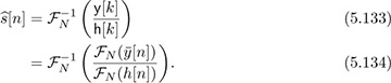
Example 5.10 To get some insight into the impact of intersymbol interference, suppose that  . Then

The nth symbol s[n] is subject to interference from s[n − 1], sent in the previous symbol period. Without correcting for this interference, detection performance will be bad. Treating ISI as noise,

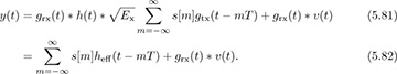
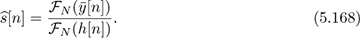
For example, for SNR = 10dB = 10 and |h1|2 = 1, SINR = 10/(10+1) = 0.91 or −0.4dB. Figure 5.16 shows the SINR as a function of |h1|2 for SNR = 10dB and SNR = 5dB.
)
Figure 5.16 The SINR as a function of |h1|2 for the discrete-time channel  in Example 5.10.
To develop receiver signal processing algorithms, it is reasonable to treat h[n] as causal and FIR. The causal assumption is reasonable because the propagation channel cannot predict the future. Furthermore, frame synchronization algorithms attempt to align, assuming a causal impulse response. The FIR assumption is reasonable because (a) there are no perfectly reflecting environments and (b) the signal energy decays as a function of distance between the transmitter and the receiver. Essentially, every time the signal reflects, some of the energy passes through the reflector or is scattered and thus it loses energy. As the signal propagates, it also loses power as it spreads in the environment. Multipaths that are weak will fall below the noise threshold. With the FIR assumption,
The channel is fully specified by the L+1 coefficients  . The order of the channel, given by L, determines to a large extent the severity of the ISI. Flat fading corresponds to the special case of L = 0. We develop equalizers specifically for the system model in (5.87), assuming that the channel coefficients are perfectly known at the receiver.
5.2.2 Linear Equalizers in the Time Domain
In this section, we develop an FIR equalizer to remove (approximately) the effects of ISI. We suppose that the channel coefficients are known perfectly; they can be estimated using training data via the method described in Section 5.3.1.
There are many strategies for equalization. One of the best approaches is to apply what is known as maximum likelihood sequence detection [348]. This is a generalization of the AWGN detection rule, which incorporates the memory in the channel due to L > 0. Unfortunately, this detector is complex to implement for channels with large L, though note that it is implemented in practical systems for modest values of L. Another approach is decision feedback equalization, where the contributions of detected symbols are subtracted, reducing the extent of the ISI [17, 30]. Combinations of these approaches are also possible.
In this section, we develop an FIR linear equalizer that operates on the time-domain signal. The goal of a linear equalizer is to find a filter that removes the effects of the channel. Let  be an FIR equalizer. The length of the equalizer is given by Lf. The equalizer is also associated with an equalizer delay nd, which is a design parameter. Generally, allowing nd > 0 improves performance. The best equalizers consider several values of nd and choose the best one.
An ideal equalizer, neglecting noise, would satisfy
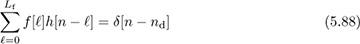
for n = 0, 1, . . . , Lf + L. Unfortunately, there are only Lf + 1 unknown parameters, so (5.88) can be satisfied exactly only in trivial cases like flat fading. This is not a surprise, as we know from DSP that the inverse of an FIR filter is an IIR filter. Alternatively, we pursue a least squares solution to (5.88).
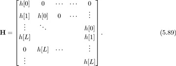
We write (5.88) as a linear system and then find the least squares solution. The key idea is to write a set of linear equations and solve for the filter coefficients that ensure that (5.88) minimizes the squared error. First incorporate the channel coefficients into the Lf + L + 1 × Lf + 1 convolution matrix:
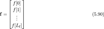
Then write the equalizer coefficients in a vector
and the desired response as the vector end with zeros everywhere except for a 1 in the nd + 1 position. With these definitions, the desired linear system is

The least squares solution is

with squared error

The squared error can be minimized further by choosing nd such that J[nd] is minimized. This is known as optimizing the equalizer delay.
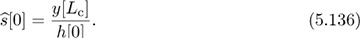
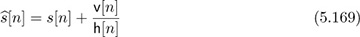
Example 5.11 In this example, we compute the least squares optimal equalizer of length Lf = 6 for a channel with impulse response h[0] = 0.5, h[1] = j/2, and h[2] = 0.4 exp(j * π/5). First we construct the convolution matrix
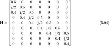
and use it to compute (5.93) to determine the optimal equalizer length. As illustrated in Figure 5.17(a), the optimum delay occurs at nd = 5 with J[5] = 0.0266. The optimum equalizer derived from (5.92) is
)
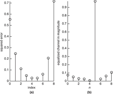
Figure 5.17 The squared error for the equalizer J[nd] in (a) and the equalized channel h[n] * fnd[n] in (b), corresponding to the parameters in Example 5.11
The equalized impulse response is plotted in Figure 5.17(b).
The matrix H has a special kind of structure. Notice that the diagonals are all constant. This is known as a Toeplitz matrix, sometimes called a filtering matrix. It shows up often when writing a convolution in matrix form. The structure in Toeplitz matrices also leads to many efficient algorithms for solving least squares equations, implementing adaptive solutions, and so on [172, 294]. This structure also means that H is full rank as long as at least one coefficient is nonzero. Therefore, the inverse in (5.92) exists.
The equalizer is applied to the sampled received signal to produce
The delay nd is known and can be corrected by advancing the output by the corresponding number of samples.
An alternative to the least squares equalizer is the LMMSE equalizer. Let us rewrite (5.96) to place the equalizer coefficients into a single vector

where yT[n] = [y[n], y[n − 1], . . . , y[n − Lf]T,

with sT[n] = [s[n], s[n − 1], . . . , s[n − L]]T and H as in (5.89). We seek the equalizer that minimizes the mean squared error

Assume that s[n] is IID with zero mean and unit variance, v[n] is IID with variance  , and s[n] and v[n] are independent. As a result,
and
Then we can apply the results from Section 3.5.4 to derive
where the conjugate results from the use of conjugate transpose in the formulation of the equalizer in (3.459). The LMMSE equalizer gives an inverse that is regularized by the noise power  , which is No if the only impairment is AWGN. This should improve performance at lower values of the SNR where equalization creates the most noise enhancement.
The asymptotic equalizer properties are interesting. As  , fnd,MMSE → fLS,nd. In the absence of noise, the MMSE solution becomes the LS solution. As
  ,
,  . This can be seen as a spatially matched filter.
A block diagram of linear equalization and channel estimation is illustrated in Figure 5.18. Note that the optimization over delay and correction for delay are included in the equalization computation, though they could be separated in additional blocks. Symbol synchronization is included in the diagram, despite the fact that linear equalization can correct for symbol timing errors through equalization. The reason is that SNR performance can nonetheless be improved by taking the best sample, especially when the pulse shape has excess bandwidth. An alternative is to implement a fractionally spaced equalizer, which operates on the signal prior to downsampling [128]. This is explored further in the problems at the end of the chapter.
)
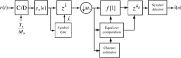
Figure 5.18 Receiver with channel estimation and linear equalization
A final comment on complexity. The length of the equalizer Lf is a design parameter that depends on L. The parameter L is the extent of the multipath in the channel and is determined by the bandwidth of the signal as well as the maximum delay spread derived from propagation channel measurements. The equalizer is an approximate FIR inverse of an FIR filter. As a consequence, performance will improve if Lf is large, assuming perfect channel knowledge. The complexity required per symbol, however, also grows with Lf. Thus there is a trade-off between choosing large Lf to have better equalizer performance and smaller Lf to have more efficient receiver implementation. A rule of thumb is to take Lf to be at least 4L.
5.2.3 Linear Equalization in the Frequency Domain with SC-FDE
Both the direct and the indirect equalizers require a convolution on the received signal to remove the effects of the channel. In practice this can be done with a direct implementation using the overlap-and-add or overlap-and-save methods for efficiently computing convolutions in the frequency domain. An alternative to FIR in the time domain is to perform equalization completely in the frequency domain. This has the advantage of allowing an ideal inverse of the channel to be computed. Application of frequency-domain equalization, though, requires additional mathematical structure in the transmitted waveform as we now explain.
In this section, we describe a technique known as SC-FDE [102]. At the transmitter, SC-FDE divides the symbols into blocks and adds redundancy in the form of a cyclic prefix. The receiver can exploit this extra information to permit equalization using the DFT. The result is an equalization strategy that is capable of perfectly equalizing the channel, in the absence of noise. SC-FDE is supported in IEEE 802.11ad, and a variation is used in the uplink of 3GPP LTE.
We now explain the motivation for working with the DFT and the key ideas behind the cyclic prefix. First, we explain why direct application of the DTFT is not feasible. Consider the received signal with intersymbol interference but without noise in (5.87). In the frequency domain

The ideal zero-forcing equalizer is

Unfortunately, it is not possible to directly implement the ideal zero-forcing equalizer in the DTFT frequency domain. First of all, the equalizer does not exist at f for which H(ej2πf) is zero. This can be solved by using a pseudo-inverse rather than an inverse equalizer. Several more important problems occur as a by-product of the use of the DTFT. It is often not possible to compute the ideal DTFT in practice. For example, the whole {s[n]} → S(ej2πf) is required, but typically only a few samples of s[n] are available. Even when {s[n]} is available, the DTFT may not even exist since the sum may not converge. Furthermore, it is not possible to observe over a long interval since h[ℓ] is time invariant only over a short window.
A solution to this problem is to use a specially designed {s[n]} and leverage the principles of the discrete Fourier transform. A comprehensive discussion of the DFT and its properties is provided in Chapter 3. To review, recall that the DFT is a basis expansion for finite-length signals:
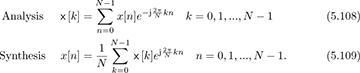
The DFT can be computed efficiently with the FFT for N as a power of 2 and certain other special cases. Practical implementations of the DFT use the FFT. The key properties of the DFT are summarized in Table 3.5.
A distinguishing feature of the DFT is that multiplication in frequency corresponds to circular convolution in time. Consider two sequences  and
and  . Let FN (·) denote the DFT operation on a length N signal, and let
  denote its inverse. With ×1[k] = FN (x1[n]) and ×2[k] = FN [x2[n]], then
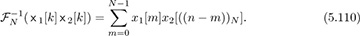
Unfortunately, linear convolution, not circular convolution, is a good model for the effects of wireless propagation per (5.87).
It is possible to mimic the effects of circular convolution by modifying the transmitted signal with a suitably chosen guard interval. The most common choice is what is called a cyclic prefix, illustrated in Figure 5.19. To understand the need for a cyclic prefix, consider the circular convolution between a block of symbols of length N where N > L:  and the channel
  , which has been zero padded to have length N, that is, h[n] = 0 for n ∈ [L + 1, N − 1]. The output of the circular convolution is
)
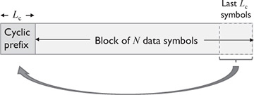
Figure 5.19 The cyclic prefix
The portion for n ≥ L looks like a linear convolution; the circular wrap-around occurs only for the first L samples.
Now we modify the transmitted sequence to obtain a circular convolution from the linear convolution introduced by the channel. Let Lc ≥ L be the length of the cyclic prefix. Form the signal 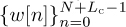 where the cyclic prefix is

and the data is

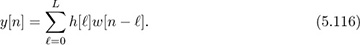
After convolution with an L + 1 tap channel, and neglecting noise for the derivation,
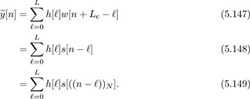
Now we neglect the first Lc terms of the convolution, which is called discarding the cyclic prefix, to form the new signal:
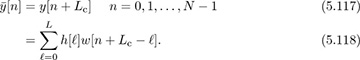
To see the effect, it is useful to evaluate  for a few values of n:
For values of n < L, the cyclic prefix replicates the effects of the linear convolution observed in (5.113). For values of N ≥ L, the circular convolution becomes a linear convolution, also as expected from (5.113) because L < N. In general, the truncated sequence satisfies
Therefore, thanks to the cyclic prefix, it is possible to implement frequency-domain equalization simply by computing  , s[k] = FN (s[n]), and then
This is the key idea behind the SC-FDE equalizer.
The cyclic prefix also acts as a guard interval, separating the contributions of different blocks of data. To see this, note that  depends only on symbols
  and not symbols sent in previous blocks like s[n] for n < 0 or n > N. Zero padding can alternatively be used as a guard interval, as explored in Example 5.12.
Example 5.12 Zero padding is an alternative to the cyclic prefix [236]. With zero padding, Lc zero values replace the cyclic prefix where

The data is encoded as in (5.115) and L ≤ Lc. We neglect noise for this problem.
Show how zero padding enables successive decoding of s[n] from y[n]. Hint: Start with n = 0 and show that s[0] can be derived from y[Lc]. Let
 denote the detected symbol. Then show how, by subtracting off
  , you can detect
  . Then assume it is true for a given n and show that it works for n + 1.
Answer: To decode s[0], we look at the expression of y[Lc]. After expanding and simplifying, because of the zeros, we obtain y[Lc] = h[0]w[Lc] = h[0]s[0]. Because h[0] is known, we can decode s[0] as
To decode s[1], we use y[Lc + 1] and the previously detected value of
 . Because
  , and assuming the detected symbol is correct,
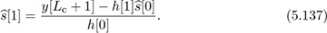
Finally, assume that
 has been decoded; then
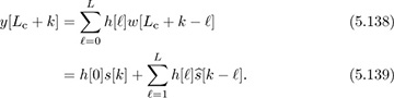
We thus can decode s[k] as follows:
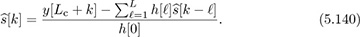
The main drawback of this approach is that it suffers from error propagation: a symbol error in
 affects the detection of all symbols after k.
Consider the following alternative to discarding the cyclic prefix:

Show how this structure also permits frequency domain equalization (neglect noise for the derivation).
Answer: For n = 0, 1, . . . , L − 1:
where the cancellation is due to the cyclic prefix. For n = L, L − 1, . . . , N − 1:
Therefore,
 is the same as (5.132), and the same equalization as SC-FDE can be applied, with a little performance penalty due to the double addition of noise. Zero padding has been used in UWB (ultra-wideband) [197] to make multiband OFDM easier to implement, and in millimeter-wave SC-FDE systems [82], where it allows for reconfiguration of the RF parameters without signal distortion.
Noise has an adverse effect on the performance of the SC-FDE equalizer. Now we examine what happens to the effective noise variance after equalization. In the presence of noise, and with perfect channel state information,

The second term is augmented during the equalization process in what is called noise enhancement. Let  be the enhanced noise component. It remains zero mean. To compute its variance, we expand the enhanced noise as
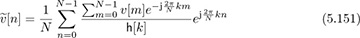
and then compute
where the results follow from the IID property of υ[n] and repeated applications of the orthogonality of discrete-time complex exponentials. The main conclusion is that we can model (5.150) as

where ν[n] is AWGN with variance given in (5.156), which is the geometric mean of the inverse of the channel in the frequency domain. We contrast this result with that obtained using OFDM in the next section.
An implementation of a QAM system with frequency-domain equalization is illustrated in Figure 5.20. The operation of collecting the input bits into groups of N symbols is given by the serial-to-parallel converter. A cyclic prefix takes the N input symbols, copies the last Lc symbols to the beginning, and outputs N + Lc symbols. The resulting symbols are then converted from parallel to serial, followed by upsampling and the usual matched filtering. The serial-to-parallel and parallel-to-serial blocks can be implemented from a DSP perspective using simple filter banks.
)
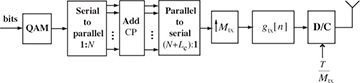
Figure 5.20 QAM transmitter for a single-carrier frequency-domain equalizer, with CP denoting cyclic prefix
Compared with linear equalization, SC-FDE has several advantages. The channel inverse can be done perfectly since the inverse is exact in the DFT domain (assuming, of course, that none of the h[k] are zero), and the time-domain equalizer is an approximate inverse. SC-FDE also works regardless of the value of L as long as Lc ≥ L. The equalizer complexity is fixed and is determined by the complexity of the FFT operation, proportional to N log2 N. The complexity of the time-domain equalizer is a function of K and generally grows with L (assuming that K grows with L), unless it is itself implemented in the frequency domain. As a general rule of thumb it becomes more efficient to equalize in the frequency domain for L around 5.
The main parameters to select in SC-FDE are N and Lc. To minimize complexity it makes sense to take N to be small. The amount of overhead, though, is Lc/(N + Lc). Consequently, taking N to be large reduces the system overhead incurred by redundancy in the cyclic prefix. Too large an N, however, may mean that the channel varies over the N symbols, violating the LTI assumption. In general, Lc is selected to be large enough that L < Lc for most channel realizations, throughout the use cases of the wireless system. For example, for a personal area network application, indoor channel measurements may be used to establish the power delay profile and other channel statistics from which a maximum value of Lc can be derived.
5.2.4 Linear Equalization in the Frequency Domain with OFDM
The SC-FDE receiver illustrated in Figure 5.21 performs a DFT on a portion of the received signal, equalizes with the DFT of the channel, and takes the IDFT (inverse discrete Fourier transform) to form the equalized sequence  . This offloads the primary equalization operations to the receiver. In some cases, however, it is of interest to have a more balanced load between transmitter and receiver. A solution is to shift the IDFT to the transmitter. This results in a framework known as multicarrier modulation or OFDM modulation [63, 72].
)
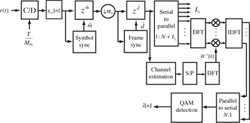
Figure 5.21 Receiver with cyclic prefix removal and a frequency-domain equalizer
Several wireless standards have adopted OFDM modulation, including wireless LAN standards like IEEE 802.11a/b/n/ac/ad [279, 290], fourth-generation cellular systems like 3GPP LTE [299, 16, 93, 253], digital audio broadcasting (DAB) [333], and digital video broadcasting (DVB) [275, 104].
In this section, we describe the key operations of OFDM at the transmitter as illustrated in Figure 5.22 and the receiver as illustrated in Figure 5.23. We present OFDM from the perspective of having already derived SC-FDE, though historically OFDM was developed several decades prior to SC-FDE. We conclude with a discussion of OFDM versus SC-FDE versus linear equalization techniques.
)
)
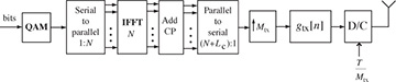
Figure 5.22 Block diagram of an OFDM transmitter. Often the upsampling and digital pulse shaping are omitted when rectangular pulse shapes are used. The inverse DFT is implemented using an inverse fast Fourier transform (IFFT).
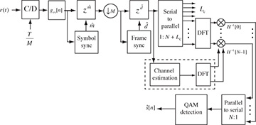
Figure 5.23 Block diagram of an OFDM receiver. Normally the matched filtering and symbol synchronization functions are omitted.
The key idea of OFDM, from the perspective of SC-FDE, is to insert the IDFT after the first serial-to-parallel converter in Figure 5.22. Given  and a cyclic prefix of length Lc, the transmitter produces the sequence

which is passed to the transmit pulse-shaping filter. The signal w[n] satisfies w[n] = w[n + N] for n = 0, 1, . . . , Lc − 1; therefore, it has a cyclic prefix. The samples {w[Lc], w[Lc + 1], . . . , w[N + Lc − 1]} correspond to the IDFT of . Unlike the SC-FDE case, the transmitted symbols can be considered to originate in the frequency domain. We do not use the frequency-domain notation for s[n] for consistency with the signal model.
We present the transmitter structure in Figure 5.22 to make the connection with SC-FDE clear. In OFDM, though, it is common to use rectangular pulse shaping where

This function is not bandlimited, so it cannot strictly speaking be implemented using the upsampling followed by digital pulse shaping as shown in Figure 5.22. Instead, it is common to simply use the “stair-step” response of the digital-to-analog converter to perform the pulse shaping. This results in a signal at the output of the DAC that takes the form
This interpretation shows how symbol s[m] rides on continuous-time carrier exp(j2πtm/NT) at baseband with a carrier of frequency 1/NT, which is also called the subcarrier bandwidth. This is one reason that OFDM is also called multicarrier modulation. We write the summation as shown in (5.160) to make it clear that frequencies around . . . , N − 3, N − 2, N − 1, 0, 1, 2, . . . are low frequencies whereas those around N/2 are high frequencies. Subcarrier n = 0 is known as the DC subcarrier, which is often assigned a zero symbol to avoid DC offset issues. The subcarriers near N/2 are often assigned zero symbols to facilitate spectral shaping.
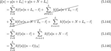
Now we show how OFDM works. Consider the received signal as in (5.116). Discard the first Lc samples to form

Inserting (5.158) for w[n] and interchanging summations gives
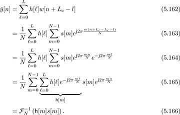
Therefore, taking the DFT gives

for n = 0, 1, . . . , N − 1, and equalization simply involves multiplying by h−1[n]. Low SNR performance could be improved by multiplying by the LMMSE equalizer  instead of by h−1[n]. In terms of time-domain quantities,
The effective channel experienced by s[n] is h[n], which is a flat-fading channel. OFDM effectively converts a problem of equalizing a frequency-selective channel into that of equalizing a set of parallel flat-fading channels. Equalization thus simplifies a great deal versus time-domain linear equalization.
The terminology in OFDM systems is slightly different from that in single-carrier systems. Usually in OFDM, the collection of samples including the cyclic prefix  is called an OFDM symbol. The constituent symbols
  are called subsymbols. The OFDM symbol period is (N + Lc)T, and T is called the sample period. The guard interval, or cyclic prefix duration, is LcT. The subcarrier spacing is 1/(NT) and is the spacing between adjacent subcarriers as measured on a spectrum analyzer. The passband bandwidth is 1/T, assuming the use of a sinc pulse-shaping filter (which is not common; a rectangular pulse shape is used along with zeroing certain subcarriers).
There are many trade-offs associated with selecting different parameters. Making N large while Lc is fixed reduces the fraction of overhead N/(N +Lc) due to the cyclic prefix. A larger N, though, means a longer block length and shorter subcarrier spacing, increasing the impact of time variation in the channel, Doppler, and residual carrier frequency offset. Complexity also increases with larger values as the complexity of processing per subcarrier grows with log2 N.
Example 5.13 Consider an OFDM system where the OFDM symbol period is 3.2µs, the cyclic prefix has length Lc = 64, and the number of subcarriers is N = 256. Find the sample period, the passband bandwidth (assuming that a sinc pulse-shaping filter is used), the subcarrier spacing, and the guard interval.
Answer: The sample period T satisfies the relation T (256 + 64) = 3.2µs, so the sample period is T = 10ns. Then, the passband bandwidth is 1/T = 100MHz. Also, the subcarrier spacing is 1/(NT) = 390.625kHz. Finally, the guard interval is LcT = 640ns.
Noise impacts OFDM differently than SC-FDE. Now we examine what happens to the effective noise variance after equalization. In the presence of noise, and with perfect channel state information,
where v[n] = FN (υ[n]). Because linear combinations of Gaussian random variables are Gaussian, and the DFT is an orthogonal transformation, v[n] remains Gaussian with zero mean and variance  . Therefore, v[n]/h[n] is AWGN with zero mean and variance
  . Unlike SC-FDE, the noise enhancement varies with different subcarriers. When h[n] is small for a particular value of n (close to a null in the spectrum), substantial noise enhancement is created. With SC-FDE there is also noise enhancement, but each detected symbol sees the same effective noise variance as in (5.156). With coding and interleaving, the error rate differences between SC-FDE and OFDM are marginal, unless other impairments like low-resolution DACs and ADCs or nonlinearities are included in the comparison (see, for example, [291, 102, 300, 192, 277]) when SC-FDE has a slight edge.
OFDM is in general more sensitive to RF impairments compared with SC-FDE and standard complex pulse-amplitude modulated signals. It is sensitive to nonlinearities because the ratio between the peak of the OFDM signal and its average value (called the peak-to-average power ratio) is higher in an OFDM system compared with a standard complex pulse-amplitude modulated signal. The reason is that the IDFT operation at the transmitter makes the signal more likely to have all peaks. Signal processing techniques can be used to mitigate some of the differences [166]. OFDM signals are also more sensitive to phase noise [264], gain and phase imbalance [254], and carrier frequency offset [75].
The OFDM waveform offers additional degrees of flexibility not found in SC-FDE. For example, the information rate can be adjusted to current channel conditions based on the frequency selectivity of the channel by changing the modulation and coding on different subcarriers. Spectral shaping is possible by zeroing certain symbols, as already described. Different users can even be allocated to subcarriers or groups of subcarriers in what is called orthogonal frequency-division multiple access (OFDMA). Many systems like IEEE 802.11a/g/n/ac use OFDM exclusively for transmission and reception. 3GPP LTE Advanced uses OFDM on the downlink and a variation of SC-FDE on the uplink where power backoff is more critical. IEEE 802.11ad supports SC-FDE as a mandatory mode and OFDM in a higher-rate optional mode. Despite their differences, both OFDM and SC-FDE maintain an important advantage of time-domain linear equalization: the equalizer complexity does not scale with L, as long as the cyclic prefix is long enough. Going forward, OFDM and SC-FDE are likely to continue to see wide commercial deployment.