Dealing with Impairments in Wireless Communication
- 5.1 Frequency-Flat Wireless Channels
- 5.2 Equalization of Frequency-Selective Channels
- 5.3 Estimating Frequency-Selective Channels
- 5.4 Carrier Frequency Offset Correction in Frequency-Selective Channels
- 5.5 Introduction to Wireless Propagation
- 5.6 Large-Scale Channel Models
- 5.7 Small-Scale Fading Selectivity
- 5.8 Small-Scale Channel Models
- 5.9 Summary
- Problems
Wireless communication is a critical discipline of electrical engineering and computer science. In this excerpt, explore channel impairments and algorithms for estimating unknown parameters to remove their effects.
Save 35% off the list price* of the related book or multi-format eBook (EPUB + MOBI + PDF) with discount code ARTICLE.
* See informit.com/terms
This chapter is from the book
This chapter is from the book
This chapter is from the book
Communication in wireless channels is complicated, with additional impairments beyond AWGN and more elaborate signal processing to deal with those impairments. This chapter develops more complete models for wireless communication links, including symbol timing offset, frame timing offset, frequency offset, flat fading, and frequency-selective fading. It also reviews propagation channel modeling, including large-scale fading, small-scale fading, channel selectivity, and typical channel models.
We begin the chapter by examining the case of frequency-flat wireless channels, including topics such as the frequency-flat channel model, symbol synchronization, frame synchronization, channel estimation, equalization, and carrier frequency offset correction. Then we consider the ramifications of communication in considerably more challenging frequency-selective channels. We revisit each key impairment and present algorithms for estimating unknown parameters and removing their effects. To remove the effects of the channel, we consider several types of equalizers, including a least squares equalizer determined from a channel estimate, an equalizer directly determined from the unknown training, single-carrier frequency-domain equalization (SC-FDE), and orthogonal frequency-division multiplexing (OFDM). Since equalization requires an estimate of the channel, we also develop algorithms for channel estimation in both the time and frequency domains. Finally, we develop techniques for carrier frequency offset correction and frame synchronization. The key idea is to use a specially designed transmit signal to facilitate frequency offset estimation and frame synchronization prior to other functions like channel estimation and equalization. The approach of this chapter is to consider specific algorithmic solutions to these impairments rather than deriving optimal solutions.
We conclude the chapter with an introduction to propagation channel models. Such models are used in the design, analysis, and simulation of communication systems. We begin by describing how to decompose a wireless channel model into two submodels: one based on large-scale variations and one on small-scale variations. We then introduce large-scale models for path loss, including the log-distance and LOS/NLOS channel models. Next, we describe the selectivity of a small-scale fading channel, explaining how to determine if it is frequency selective and how quickly it varies over time. Finally, we present several small-scale fading models for both flat and frequency-selective channels, including some analysis of the effects of fading on the average probability of symbol error.
5.1 Frequency-Flat Wireless Channels
In this section, we develop the frequency-flat AWGN communication model, using a single-path channel and the notion of the complex baseband equivalent. Then we introduce several impairments and explain how to correct them. Symbol synchronization corrects for not sampling at the correct point, which is also known as symbol timing offset. Frame synchronization finds a known reference point in the data—for example, the location of a training sequence—to overcome the problem of frame timing offset. Channel estimation is used to estimate the unknown flat-fading complex channel coefficient. With this estimate, equalization is used to remove the effects of the channel. Carrier frequency offset synchronization corrects for differences in the carrier frequencies between the transmitter and the receiver. This chapter provides a foundation for dealing with impairments in the more complicated case of frequency-selective channels.
5.1.1 Discrete-Time Model for Frequency-Flat Fading
The wireless communication channel, including all impairments, is not well modeled simply by AWGN. A more complete model also includes the effects of the propagation channel and filtering in the analog front end. In this section, we consider a single-path channel with impulse response

Based on the derivations in Section 3.3.3 and Section 3.3.4, this channel has a complex baseband equivalent given by

and pseudo-baseband equivalent channel

See Example 3.37 and Example 3.39 to review this calculation. The Bsinc(t) term is present because the complex baseband equivalent is a baseband bandlimited signal. In the frequency domain

we observe that |H(f)| is a constant for f ∈ [−B/2, B/2]. This channel is said to be frequency flat because it is constant over the bandwidth of interest to the signal. Channels that consist of multipaths can be approximated as frequency flat if the signal bandwidth is much less than the coherence bandwidth, which is discussed further in Section 5.8.
Now we incorporate this channel into our received signal model. The channel in (5.2) convolves with the transmitted signal prior to the noise being added at the receiver. As a result, the complex baseband received signal prior to matched filtering and sampling is
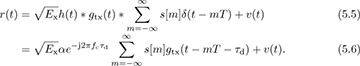
To ensure that r(t) is bandlimited, henceforth we suppose that the noise has been lowpass filtered to have a bandwidth of B/2. For simplicity of notation, and to be consistent with the discrete-time representation, we let 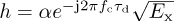 and write

The factor of  is included in h since only the combined scaling is important from the perspective of receiver design. Matched filtering and sampling at the symbol rate give the received signal

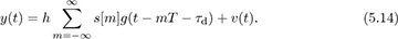
where g(t) is a Nyquist pulse shape. Compared with the AWGN received signal model y[n] = s[n] + υ[n], there are several sources of distortion, which must be recognized and corrected.
One impairment is caused by symbol timing error. Suppose that τd is a fraction of a symbol period, that is, τd ∈ [0, T). This models the effect of sample timing error, which happens when the receiver does not sample at precisely the right point in time. Under this assumption
Intersymbol interference is created when the Nyquist pulse shape is not sampled exactly at nT, since g(nT + τd) is not generally equal to δ[n]. Correcting for this fractional delay requires symbol synchronization, equalization, or a more complicated detector.
A second impairment occurs with larger delays. For illustration purposes, suppose that τd = dT for some integer d. This is the case where symbol timing has been corrected but an unknown propagation delay, which is a multiple of the symbol period, remains. Under this assumption
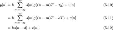
Essentially integer offsets create a mismatch between the indices of the transmitted and received symbols. Frame synchronization is required to correct this frame timing error impairment.
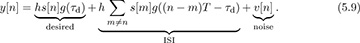
Finally, suppose that the unknown delay τd has been completely removed so that τd = 0. Then the received signal is

Sampling and removing delay leaves distortion due to the attenuation and phase shift in h. Dealing with h requires either a specially designed modulation scheme, like DQPSK (differential quadrature phase-shift keying), or channel estimation and equalization.
It is clear that amplitude, phase, and delay if not compensated can have a drastic impact on system performance. As a consequence, every wireless system is designed with special features to enable these impairments to be estimated or directly removed in the receiver processing. Most of this processing is performed on small segments of data called bursts, packets, or frames. We emphasize this kind of batch processing in this book. Many of the algorithms have adaptive extensions that can be applied to continually estimate impairments.
5.1.2 Symbol Synchronization
The purpose of symbol synchronization, or timing recovery, is to estimate and remove the fractional part of the unknown delay τd, which corresponds to the part of the error in [0, T). The theory behind these algorithms is extensive and their history is long [309, 226, 124]. The purpose of this section is to present one of the many algorithm approaches for symbol synchronization in complex pulse-amplitude modulated systems.
Philosophically, there are several approaches to synchronization as illustrated in Figure 5.1. There is a pure analog approach, a combined digital and analog approach where digital processing is used to correct the analog, and a pure digital approach. Following the DSP methodology, this book considers only the case of pure digital symbol synchronization.
)
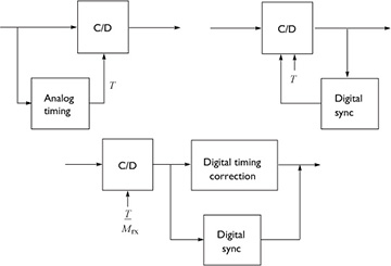
FIGURE 5.1 Different options for correcting symbol timing. The bottom approach relies only on DSP.
We consider two different strategies for digital symbol synchronization, depending on whether the continuous-to-discrete converter can be run at a low sampling rate or a high sampling rate:
The oversampling method, illustrated in Figure 5.2, is suitable when the oversampling factor Mrx is large and therefore a high rate of oversampling is possible. In this case the synchronization algorithm essentially chooses the best multiple of T/Mrx and adds a suitable integer delay k* prior to downsampling.
The resampling method is illustrated in Figure 5.3. In this case a resampler, or interpolator, is used to effectively create an oversampled signal with an effective sample period of T/Mrx even if the actual sampling is done with a period less than T/Mrx but still satisfying Nyquist. Then, as with the oversampling method, the multiple of T/Mrx is estimated and a suitable integer delay k* is added prior to the downsampling operation.
)
)
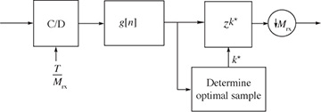
FIGURE 5.2 Oversampling method suitable when Mrx is large
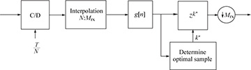
FIGURE 5.3 Resampling or interpolation method suitable when Mrx is small, for example, N = 2
A proper theoretical approach for solving for the best of τd would be to use estimation theory. For example, it is possible to solve for the maximum likelihood estimator. For simplicity, this section considers an approach based on a cost function known as the maximum output energy (MOE) criterion, the same approach as in [169]. There are other approaches based on maximum likelihood estimation such as the early-late gate approach. Lower-complexity implementations of what is described are possible that exploit filter banks; see, for example, [138].
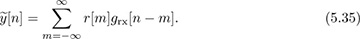
First we compute the energy output as a way to justify each approach for timing synchronization. Denote the continuous-time output of the matched filter as
The output energy after sampling by nT + τ is
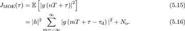
Suppose that τd = dT + τfrac and 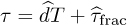 ; then
with a change of variables. Therefore, while the delay τ can take an arbitrary positive value, only the offset that corresponds to the fractional delay has an impact on the output energy.
The maximum output energy approach to symbol timing attempts to find the τ that maximizes JMOE(τ) where τ ∈ [0, T]. The maximum output energy solution is

The rationale behind this approach is that

where the inequality is true for most common pulse-shaping functions (but not for arbitrarily chosen pulse shapes). Thus the unique maximum of JMOE(τ) corresponds to τ = τd. The values of JMOE(τ) are plotted in Figure 5.4 for the raised cosine pulse shape. A proof of (5.20) for sinc and raised cosine pulse shapes is established in Example 5.1 and Example 5.2.
)
FIGURE 5.4 Plot of JMOE(τ) for τ ∈ [−T/2, T/2], in the absence of noise, assuming a raised cosine pulse shape (4.73). The x-axis is normalized to T. As the rolloff value of the raised cosine is increased, the output energy peaks more, indicating that the excess bandwidth provided by choosing larger values of rolloff α translates into better symbol timing using the maximum output energy cost function.
Example 5.1 Show that the inequality in (5.20) is true for sinc pulse shapes.
Answer: For convenience denote

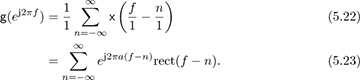
where  . Let g(t) = sinc(t+a) and g[m] = g(mT) = sinc(m+a), and let g(f) and g(ej2πf) be the CTFT of g(t) and DTFT of g[m] respectively. Then g(f) = ej2πaf rect(f) and
By Parseval’s theorem for the DTFT we have
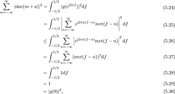
where the inequality follows because |∑ai| ≤ ∑ |ai|. Therefore,
Example 5.2 Show that the MOE inequality in (5.20) holds for raised cosine pulse shapes.
Answer: The raised cosine pulse

is a modulated version of the sinc pulse shape. Since
it follows that

and the result from Example 5.1 can be used.
Now we develop the direct solution to maximizing the output energy, assuming the receiver architecture with oversampling as in Figure 4.10. Let r[n] denote the signal after oversampling or resampling, assuming there are Mrx samples per symbol period. Let the output of the matched receiver filter prior to downsampling at the symbol rate be
We use this sampled signal to compute a discrete-time version of JMOE(τ) given by

where k is the sample offset between 0, 1, . . . , Mrx − 1 corresponding to an estimate of the fractional part of the timing offset given by kT/Mrx. To develop a practical algorithm, we replace the expectation with a time average over P symbols, thanks to ergodicity, so that
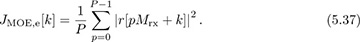
Looking for the maximizer of JMOE,e[k] over k = 0, 1, . . . , Mrx − 1 gives the optimum sample k* and an estimate of the symbol timing offset k*T/Mrx.
The optimum correction involves advancing the received signal by k* samples prior to downsampling. Essentially, the synchronized data is 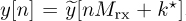 . Equivalently, the signal can be delayed by k* − Mrx samples, since subsequent signal processing steps will in any case correct for frame synchronization.
The main parameter to be selected in the symbol timing algorithms covered in this section is the oversampling factor Mrx. This decision can be based on the residual ISI created because the symbol timing is quantized. Using the SINR from (4.56), assuming h is known perfectly, matched filtering at the receiver, and a maximum symbol timing offset T/2Mrx, then
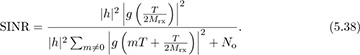
This value can be used, for example, with the probability of symbol error analysis in Section 4.4.5 to select a value of Mrx such that the impact of symbol timing error is acceptable, depending on the SNR and target probability of symbol error. An illustration is provided in Figure 5.5 for the case of 4-QAM. In this case, a value of Mrx = 8 leads to less than 1dB of loss at a symbol error rate of 10−4.
)
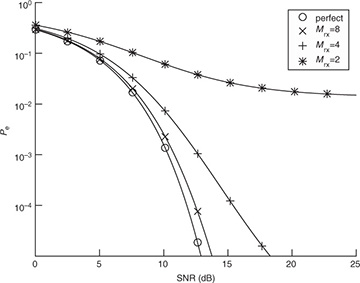
FIGURE 5.5 Plot of the exact symbol error rate for 4-QAM from (4.147), substituting SINR for SNR, with  for different values of Mrx in (5.38), assuming a raised cosine pulse shape with α = 0.25. With enough oversampling, the effects of timing error are small.
5.1.3 Frame Synchronization
The purpose of frame synchronization is to resolve multiple symbol period delays, assuming that symbol synchronization has already been performed. Let d denote the remaining offset where d = τd/T − k*/Mrx, assuming the symbol timing offset was corrected perfectly. Given that, ISI is eliminated and

To reconstruct the transmitted bit sequence it is necessary to know “where the symbol stream starts.” As with symbol synchronization, there is a great deal of theory surrounding frame synchronization [343, 224, 27]. This section considers one common algorithm for frame synchronization in flat channels that exploits the presence of a known training sequence, inserted during a training phase.
Most wireless systems insert reference signals into the transmitted waveform, which are known by the receiver. Known information is often called a training sequence or a pilot symbol, depending on how the known information is inserted. For example, a training sequence may be inserted at the beginning of a transmission as illustrated in Figure 5.6, or a few pilot symbols may be inserted periodically. Most systems use some combination of the two where long training sequences are inserted periodically and shorter training sequences (or pilot symbols) are inserted more frequently. For the purpose of explanation, it is assumed that the desired frame begins at discrete time n = 0. The total frame length is Ntot, including a length Ntr training phase and an Ntot − Ntr data phase. Suppose that  is the training sequence known at the receiver.
)
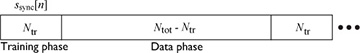
FIGURE 5.6 A frame structure that consists of periodically inserted training and data
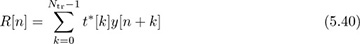
One approach to performing frame synchronization is to correlate the received signal with the training sequence to compute
and then to find

The maximization usually occurs by evaluating R[n] over a finite set of possible values. For example, the analog hardware may have a carrier sense feature that can determine when there is a significant signal of interest. Then the digital hardware can start evaluating the correlation and looking for the peak. A threshold can also be used to select the starting point, that is, finding the first value of n such that |R[n]| exceeds a target threshold. An example with frame synchronization is provided in Example 5.3.
Example 5.3 Consider a system as described by (5.39) with 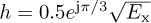 , Ntr = 7, and Ntot = 21 with d = 0. We assume 4-QAM for the data transmission and that the training consists of the Barker code of length 7 given by
  . The SNR is 5dB. We consider a frame snippet that consists of 14 data symbols, 7 training symbols, 14 data symbols, 7 training symbols, and 14 data symbols. In Figure 5.7, we plot |R[n]| computed from (5.40). There are two peaks that correspond to locations of our training data. The peaks happen at 21 and 42 as expected. If the snippet was delayed, then the peaks would shift accordingly.
)
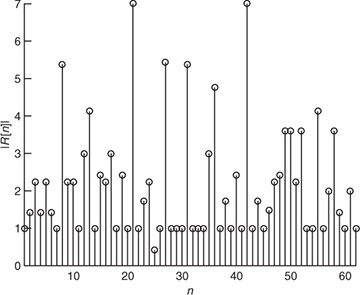
FIGURE 5.7 The absolute value of the output of a correlator for frame synchronization. The details of the simulation are provided in Example 5.3. Two correlation peaks are seen, corresponding to the location of the two training sequences.
A block diagram of a receiver including both symbol synchronization and frame synchronization operations is illustrated in Figure 5.8. The frame synchronization happens after the downsampling and prior to the symbol detection. Fixing the frame synchronization requires advancing the signal by  symbols.
)
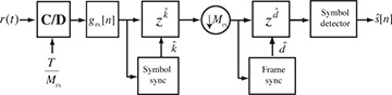
FIGURE 5.8 Receiver with symbol synchronization based on oversampling and frame synchronization
The frame synchronization algorithm may find a false peak if the data is the same as the training sequence. There are several approaches to avoid this problem. First, training sequences can be selected that have good correlation properties. There are many kinds of sequences known in the literature that have good autocorrelation properties [116, 250, 292], or periodic autocorrelation properties [70, 267]. Second, a longer training sequence may be used to reduce the likelihood of a false positive. Third, the training sequence can come from a different constellation than the data. This was used in Example 5.3 where a BPSK training sequence was used but the data was encoded with 4-QAM. Fourth, the frame synchronization can average over multiple training periods. Suppose that the training is inserted every Ntot symbols. Averaging over P periods then leads to an estimate
Larger amounts of averaging improve performance at the expense of higher complexity and more storage requirements. Finally, complementary training sequences can be used. In this case a pair of training sequences {t1[n]} and {t2[n]} are designed such that  has a sharp correlation peak. Such sequences are discussed further in Section 5.3.1.
5.1.4 Channel Estimation
Once frame synchronization and symbol synchronization are completed, a good model for the received signal is

The two remaining impairments are the unknown flat channel h and the AWGN υ[n]. Because h rotates and scales the constellation, the channel must be estimated and either incorporated into the detection process or removed via equalization.
The area of channel estimation is rich and the history long [40, 196, 369]. In general, a channel estimation problem is handled like any other estimation problem. The formal approach is to derive an optimal estimator under assumptions about the signal and noise. Examples include the least squares estimator, the maximum likelihood estimator, and the MMSE estimator; background on these estimators may be found in Section 3.5.
In this section we emphasize the use of least squares estimation, which is also the ML estimator when used for linear parameter estimation in Gaussian noise. To use least squares, we build a received signal model from (5.43) by exploiting the presence of the known training sequence from n = 0, 1, . . . , Ntr − 1. Stacking the observations in (5.43) into vectors,
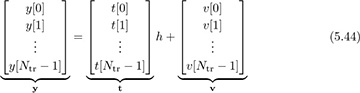
which becomes compactly

We already computed the maximum likelihood estimator for a more general version of (5.46) in Section 3.5.3. The solution was the least squares estimate, given by
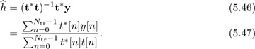
Essentially, the least squares estimator correlates the observed data with the training data and normalizes the result. The denominator is just the energy in the training sequence, which can be precomputed and stored offline. The numerator is calculated as part of the frame synchronization process. Therefore, frame synchronization and channel estimation can be performed jointly. The receiver, including symbol synchronization, frame synchronization, and channel estimation, is illustrated in Figure 5.9.
)
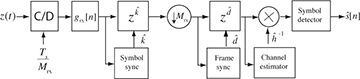
FIGURE 5.9 Receiver with symbol synchronization based on oversampling, frame synchronization, and channel estimation
Example 5.4 In this example, we evaluate the squared error in the channel estimate. We consider a similar system to the one described in Example 5.3 with a length Ntr = 7 Barker code used for a training sequence, and a least squares channel estimator as in (5.46). We perform a Monte Carlo estimate of the channel by generating a noise realization and estimating the channel  for n = 1, 2, . . . , 1000 realizations. In Figure 5.10, we evaluate the estimation error as a function of the SNR, which is defined as
  , and is 5dB in this example. We plot the error for one realization of a channel estimation, which is given by
  , and the mean squared error, which is given by
 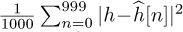 . The plot shows how the estimation error, based both on one realization and on average, decreases with SNR.
)
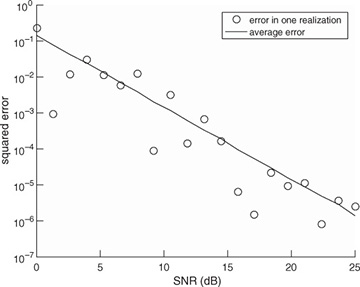
FIGURE 5.10 Estimation error as a function of SNR for the system in Example 5.4. The error estimate reduces as SNR increases.
Example 5.5 In this example, we evaluate the squared error in the channel estimate for different lengths of 4-QAM training sequences, an SNR of 5dB, the channel as in Example 5.3, and a least squares channel estimator as in (5.46). We perform a Monte Carlo estimate of the squared error of one realization and the mean squared error, as described in Example 5.4. We plot the results in Figure 5.11, which show how longer training sequences reduce estimation error. Effectively, longer training increases the effective SNR through the addition of energy through coherent combining in 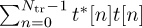 and more averaging in
 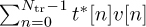 .
.
)
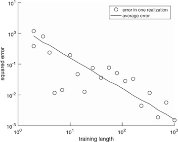
FIGURE 5.11 Estimation error as a function of the training length for the system in Example 5.5. The error estimate reduces as the training length increases.
5.1.5 Equalization
Assuming that channel estimation has been completed, the next step in the receiver processing is to use the channel estimate to perform symbol detection. There are two reasonable approaches; both involve assuming that  is the true channel estimate. This is a reasonable assumption if the channel estimation error is small enough.
The first approach is to incorporate  into the detection process. Replacing
  by h in (4.105), then

Consequently, the channel estimate becomes an input into the detector. It can be used as in (5.48) to scale the symbols during the computation of the norm, or it can be used to create a new constellation 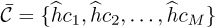 and detection performed using the scaled constellation as

The latter approach is useful when Ntot is large.
An alternative approach to incorporating the channel into the ML detector is to remove the effects of the channel prior to detection. For  ,
,

The process of creating the signal  is an example of equalization. When equalization is used, the effects of the channel are removed from y[n] and a standard detector can be applied to the result, leveraging constellation symmetries to reduce complexity. The receiver, including symbol synchronization, frame synchronization, channel estimation, and equalization, is illustrated in Figure 5.9.
The probability of symbol error with channel estimation can be computed by treating the estimation error as noise. Let  where
where  is the estimation error. For a given channel h and estimate the equalized received signal is
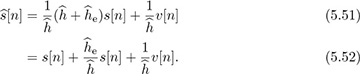
It is common to treat the middle interference term as additional noise. Moving the common  to the numerator,
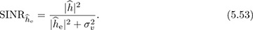
This can be used as part of a Monte Carlo simulation to determine the impact of channel estimation. Since the receiver does not actually know the estimation error, it is also common to consider a variation of the SINR expression where the variance of the estimate  is used in place of the instantaneous value (assuming that the estimator is unbiased so zero mean). Then the SINR becomes
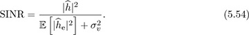
This expression can be used to study the impact of estimation error on the probability of error, as the mean squared error of the estimate is a commonly computed quantity. A comparison of the probability of symbol error for these approaches is provided in Example 5.6.
Example 5.6 In this example we evaluate the impact of channel estimation error. We consider a system similar to the one described in Example 5.4 with a length Ntr = 7 Barker code used for a training sequence, and a least squares channel estimator as in (5.46). We perform a Monte Carlo estimate of the channel by generating a noise realization and estimating the channel  for n = 1, 2, . . . , 1000 realizations. For each realization, we compute the error, insert into the
  in (5.53), and use that to compute the exact probability of symbol error from Section 4.4.5. We then average this over 1000 Monte Carlo simulations. We also compare in Figure 5.12 with the probability of error assuming no estimation error with SNR |h|2Ex/No and with the probability of error computed using the average error from the SINR in (5.54). We see in this example that the loss due to estimation error is about 1dB and that there is little difference in the average probability of symbol error and the probability of symbol error computed using the average estimation error.
)
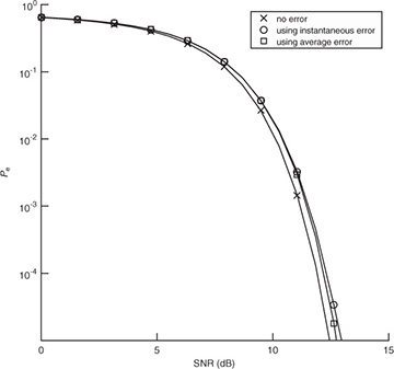
FIGURE 5.12 The probability of symbol error with 4-QAM and channel estimation using a length Ntr = 7 training sequence. The probability of symbol error with no channel estimation error is compared with the average of the probability of symbol error including the instantaneous error, and the probability of symbol error using the average estimation error. There is little loss in using the average estimation error.
5.1.6 Carrier Frequency Offset Synchronization
Wireless communication systems use passband communication signals. They can be created at the transmitter by upconverting a complex baseband signal to carrier fc and can be processed at the receiver to produce a complex baseband signal by downconverting from a carrier fc. In Section 3.3, the process of upconversion to carrier fc, downconversion to baseband, and the complex equivalent notation were explained under the important assumption that fc is known perfectly at both the transmitter and the receiver. In practice, fc is generated from a local oscillator. Because of temperature variations and the fact that the carrier frequency is generated by a different local oscillator and transmitter and receiver, in practice fc at the transmitter is not equal to  at the receiver as illustrated in Figure 5.13. The difference between the transmitter and the receiver
 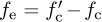 is the carrier frequency offset (or simply frequency offset) and is generally measured in hertz. In device specification sheets, the offset is often measured as |fe|/fc and is given in units of parts per million. In this section, we derive the system model for carrier frequency offset and present a simple algorithm for carrier frequency offset estimation and correction.
)
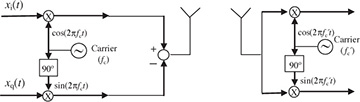
FIGURE 5.13 Abstract block diagram of a wireless system with different carrier frequencies at the transmitter and the receiver
Let

be the passband signal generated at the transmitter. Let the observed passband signal at the receiver at carrier fc be
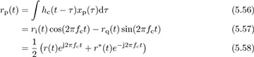
where r(t) = ri(t) + jrq(t) is the complex baseband signal that corresponds to rp(t) and we use the fact that 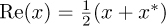 for the last step. Now suppose that rp(t) is downconverted using carrier
  to produce a new signal r′(t). Then the extracted complex baseband signal is (ignoring noise)

Focusing on the last term in (5.59) with 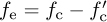 , then
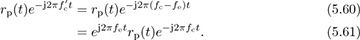
Substituting in rp(t) from (5.58),

Lowpass filtering (assuming, strictly speaking, a bandwidth of B + |fe|) and correcting for the factor of  leaves the complex baseband equivalent

Carrier frequency offset results in a rolling phase shift that happens after the convolution and depends on the difference in carrier fe. As the phase shift accumulates, failing to synchronize can quickly lead to errors.
Following the methodology of this book, it is of interest to formulate and solve the frequency offset estimation and correction problem purely in discrete time. To that end a discrete-time complex baseband equivalent model is required.
To formulate a discrete-time model, we focus on the sampled signal after matched filtering, still neglecting noise, as
Suppose that the frequency offset fe is sufficiently small that the variation over the duration of grx(t) can be assumed to be a constant; then e−j2πfeτgrx(τ) ≈ grx(τ). This is reasonable since most of the energy in the matched filter grx(t) is typically concentrated over a few symbol periods. Assuming this holds,

As a result, it is reasonable to model the effects of frequency offset as if they occurred on the matched filtered signal.
Now we specialize to the case of flat-fading channels. Substituting for r(t), adding noise, and sampling gives

where  = feT is the normalized frequency offset. Frequency offset introduces a multiplication by the discrete-time complex exponential ej2πfeTn.
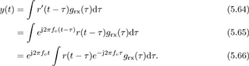
To visualize the effects of frequency offset, suppose that symbol and frame synchronization has been accomplished and only equalization and channel estimation remain. Then the Nyquist property of the pulse shape can be exploited so that

Notice that the transmit symbol is being rotated by exp(j2πn). As n increases, the offset increases, and thus the symbol constellation rotates even further. The impact of this is an increase in the number of symbol errors as the symbols rotate out of their respective Voronoi regions. The effect is illustrated in Example 5.7.
Example 5.7 Consider a system with the frequency offset described by (5.69). Suppose that = 0.05. In Figure 5.14, we plot a 4-QAM constellation at times n = 0, 1, 2, 3. The Voronoi regions corresponding to the unrotated constellation are shown on each plot as well. To make seeing the effect of the rotation easier, one point is marked with an x. Notice how the rotations are cumulative and eventually the constellation points completely leave their Voronoi regions, which results in detection errors even in the absence of noise.
)
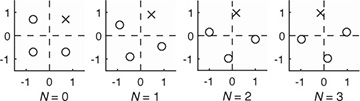
FIGURE 5.14 The successive rotation of a 4-QAM constellation due to frequency offset. The Voronoi regions for each constellation point are indicated with the dashed lines. To make the effects of the rotation clearer, one of the constellation points is marked with an x.
Correcting for frequency offset is simple: just multiply y[n] by e−j2πn. Unfortunately, the offset is unknown at the receiver. The process of correcting for is known as frequency offset synchronization. The typical method for frequency offset synchronization involves first estimating the offset  , then correcting for it by forming the new sequence
  with the phase removed. There are several different methods for correction; most employ a frequency offset estimator followed by a correction phase. Blind offset estimators use some general properties of the received signal to estimate the offset, whereas non-blind estimators use more specific properties of the training sequence.
Now we review two algorithms for correcting the frequency offset in a flat-fading channel. We start by observing that frequency offset does not impact symbol synchronization, since the ej2πfeTn cancels out the maximum output energy maximization caused by the magnitude function (see, for example, (5.15)). As a result, ISI cancels and a good model for the received signal is

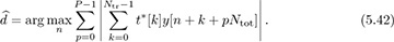
where the offset , the channel h, and the frame offset d are unknowns. In Example 5.8, we present an estimator based on a specific training sequence design. In Example 5.9, we use properties of 4-QAM to develop a blind frequency offset estimator. We compare their performance to highlight differences in the proposed approaches in Figure 5.15. We also explain how to jointly estimate the delay and channel with each approach. These algorithms illustrate some ways that known information or signal structure can be exploited for estimation.
)
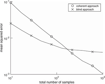
Figure 5.15 The mean squared error performance of two different frequency offset estimators: the training-based approach in Example 5.8 and the blind approach in Example 5.9. Frame synchronization is assumed to have been performed already for the coherent approach. The channel is the same as in Example 5.3 and other examples, and the SNR is 5dB. The true frequency offset is = 0.01. The estimators are compared assuming the number of samples (Ntr for the coherent case and Ntot for the blind case). The error in each Monte Carlo simulation is computed from phase  to avoid any phase wrapping effects.
Example 5.8 In this example, we present a coherent frequency offset estimator that exploits training data. We suppose that frame synchronization has been solved. Let us choose as a training sequence t[n] = exp(j2πftn) for n = 0, 1, . . . , Ntr − 1 where ft is a fixed frequency. This kind of structure is available from the Frequency Correction Burst in GSM, for example [100]. Then for n = 0, 1, . . . , Ntr − 1,

Correcting the known offset introduced by the training data gives

The rotation by e−j2πftn does not affect the distribution of the noise. Solving for the unknown frequency in (5.72) is a classic problem in signal processing and single-tone parameter estimation, and there are many approaches [330, 3, 109, 174, 212, 218]. We explain the approach used in [174] based on the model in [330]. Approximate the corrected signal in (5.72) as

where θ is the phase of h and ν[n] is Gaussian noise. Then, looking at the phase difference between two adjacent samples, a linear system can be written from the approximate model as

Aggregating the observations in (5.79) from n = 1, . . . , Ntot − 1, we can create a linear estimation problem

where [p]n = phase(ej2πftny*[n]e−j2πft(n+1)y[n + 1]), 1 is an Ntr − 1 × 1 vector, and ν is an Ntr − 1 × 1 noise vector. The least squares solution is given by
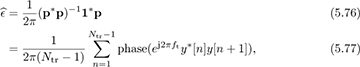
which is also the maximum likelihood solution if ν[n] is assumed to be IID [174].
Frame synchronization and channel estimation can be incorporated into this estimator as follows. Given that the frequency offset estimator in (5.77) solves a least squares problem, there is a corresponding expression for the squared error; see, for example, (3.426). Evaluate this expression for many possible delays and choose the delay that has the lowest squared error. Correct for the offset and delay, then estimate the channel as in Section 5.1.4.
Example 5.9 In this example, we exploit symmetry in the 4-QAM constellation to develop a blind frequency offset estimator, which does not require training data. The main observation is that for 4-QAM, the normalized constellation symbols are points on the unit circle. In particular for 4-QAM, it turns out that s4[n] = −1. Taking the fourth power,

where ν[n] contains noise and products of the signal and noise. The unknown parameter d disappears because s4[n − d] = −1, assuming a continuous stream of symbols. The resulting equation has the form of a complex sinusoid in noise, with unknown frequency, amplitude, and phase similar to (5.72). Then a set of linear equations can be written from

in a similar fashion to (5.75), and then
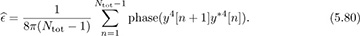
Frame synchronization and channel estimation can be incorporated as follows. Use all the data to estimate the carrier frequency offset from (5.80). Then correct for the offset and perform frame synchronization and channel estimation based on training data, as outlined in Section 5.1.3 and Section 5.1.4.