Dealing with Impairments in Wireless Communication

This chapter is from the book

Introduction to Wireless Digital Communication: A Signal Processing Perspective

Learn More Buy

This chapter is from the book

This chapter is from the book 

Introduction to Wireless Digital Communication: A Signal Processing Perspective

Learn More Buy

Problems

1. Re-create the results from Figure 5.5 but with 16-QAM. Also determine the smallest value of M_rx such that 16-QAM has a 1dB loss at a symbol error rate of 10⁻⁴.

2. Re-create the results from Example 5.3 assuming training constructed from Golay sequences as [a₈; b₈], followed by 40 randomly chosen 4-QAM symbols. Explain how to modify the correlator to exploit properties of the Golay complementary pair. Compare your results.

3. Consider the system

   

   where s[n] is a zero-mean WSS random process with correlation r_ss[n], υ[n] is a zero-mean WSS random process with correlation r_υυ[n], and s[n] and υ[n] are uncorrelated. Find the linear MMSE equalizer g such that the mean squared error is minimized:

   

   1. Find an equation for the MMSE estimator g.

   2. Find an equation for the mean squared error (substitute your estimator in and compute the expectation).

   3. Suppose that you know r_ss[n] and you can estimate r_yy[n] from the received data. Show how to find r_υυ[n] from r_ss[n] and r_yy[n].

   4. Suppose that you estimate r_yy[n] through sample averaging of N samples, exploiting the ergodicity of the process. Rewrite the equation for g using this functional form.

   5. Compare the least squares and the MMSE equalizers.

4. Consider a frequency-flat system with frequency offset. Suppose that 16-QAM modulation is used and that the received signal is

   

   where = f_offsetT_s and exp(j2πn) is unknown to the receiver. Suppose that the SNR is 10dB and the packet size is N = 101 symbols. The effect of is to rotate the actual constellation.

   1. Consider y[0] and y[1] in the absence of noise. Illustrate the constellation plot for both cases and discuss the impact of on detection.

   2. Over the whole packet, where is the worst-case rotation?

   3. Suppose that is small enough that the worst-case rotation occurs at symbol 100. What is the value of such that the rotation is greater than π/2? For the rest of this problem assume that is less than this value.

   4. Determine the such that the symbol error rate is 10⁻³. To proceed, first find an expression for the probability of symbol error as a function of . Make sure that is included somewhere in the expression. Set equal to 10⁻³ and solve.

5. Let T be a Toeplitz matrix and let T* be its Hermitian conjugate. If T is either square or tall and full rank, prove that T*T is an invertible square matrix.

6. Consider the training structure in Figure 5.37. Consider the problem of estimating the channel from the first period of training data. Let s[0], s[1], . . . , s[N_tr−1] denote the training symbols, and let s[N_tr], s[N_t + 1], . . . , s[N − 1] denote the unknown QAM data symbols. Suppose that we can model the channel as a frequency-selective channel with coefficients h[0], h[1], . . . , h[ℓ]. The received signal (assuming synchronization has been performed) is

   
   

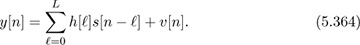
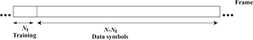
   Figure 5.37 A frame structure with a single training sequence of length N_t followed by N − N_t data symbols

   1. Write the solution for the least squares channel estimate from the training data. You can use matrices in your answer. Be sure to label the size of the matrices and their contents very carefully. Also list any critical assumptions necessary for your solution.

   2. Now suppose that the estimated channel is used to estimate an equalizer that is applied to y[n], then passed to the detector to generate tentative symbol decisions. We would like to improve the detection process by using a decision-directed channel estimate. Write the solution for the least squares channel estimate from the training data and tentative symbol decisions.

   3. Draw a block diagram for the receiver that includes synchronization, channel estimation from training, equalization, reestimation of the channel, reequalization, and the additional detection phase.

   4. Intuitively, explain how the decision-directed receiver should perform relative to only training as a function of SNR (low, high) and N_tr (small, large). Is there a benefit to multiple iterations? Please justify your answer.

7. Let be the Toeplitz matrix that is used in computing the least squares equalizer . Prove that if , is full rank.

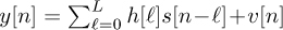
8. Consider a digital communication system where the same transmitted symbol s[n] is repeated over two different channels. This is called repetition coding. Let h₁ and h₂ be the channel coefficients, assumed to be constant during each time instance and estimated perfectly. The received signals are corrupted by υ₁[n] and υ₂[n], which are zero-mean circular symmetric complex AWGN of the same variance σ², that is, υ₁[n], υ₂[n] ~ N_c(0, σ²). In addition, s[n] has zero mean and . We assume that s[n], υ₁[n], and υ₂[n] are uncorrelated with each other. The received signals on the two channels are given by

   

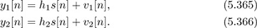
   Suppose that we use the equalizers g₁ and g₂ for the two time instances, where g₁ and g₂ are complex numbers such that |g₁|² + |g₂|² = 1. The combined signal, denoted as z[n], is formed by summing the equalized signals in two time instances:

   

   If we define the following vectors:

   

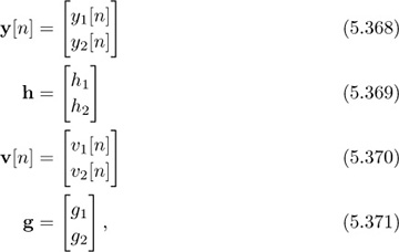
   then

   

   and

   

   1. Write an expression for z[n], first in terms of the vectors h and g, then in terms of g₁, g₂, h₁, and h₂. Thus you will have two equations for z[n].

   2. Compute the mean and the variance of the noise component in the combined signal z[n]. Remember that the noise is Gaussian and uncorrelated.

   3. Compute the SNR of the combined signal z[n] as a function of σ, h₁, h₂, g₁, and g₂ (or σ, h, and g). In this case the SNR is the variance of the combined received signal divided by the variance of the noise term.

   4. Determine g₁ and g₂ as functions of h₁ and h₂ (or g as a function of h) to maximize the SNR of the combined signal. Hint: Recall the Cauchy-Schwarz inequality for vectors and use the conditions when equality holds.

   5. Determine a set of equations for finding the LMMSE equalizers g₁ and g₂ to minimize the mean squared error, which is defined as follows:

      

      Simplify your equation by exploiting the orthogonality principle but do not solve for the unknown coefficients yet. Hints: Using the vector format might be useful, and you can assume you can interchange expectation and differentiation. First, expand the absolute value, then take the derivative with respect to g* and set the result equal to zero. Simplify as much as possible to get an expression of g as a function of h₁, h₂, and σ.

   6. The autocorrelation matrix R_yy[0] of y[n] is defined as

      

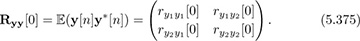
      Compute R_yy[0] as a function of σ, h₁, and h₂. Hint: and for random processes a[n] and b[n].

   7. Now solve the set of equations you formulated in part (e).

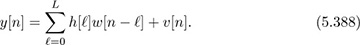
9. Consider an order L-tap frequency-selective channel. Given a symbol period of T and after oversampling with factor M_rx and matched filtering, the received signal is

   

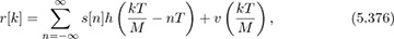
   where s is the transmitted symbols and υ is AWGN. Suppose a fractionally spaced equalizer (FSE) is applied to the received signal before downsampling. The FSE f[k] is an FIR filter with tap spacing of T/M_rx and length MN. Figure 5.38 gives the block diagram of the system.

   

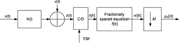
   Figure 5.38 Block diagram of a receiver with FSE

   1. Give an expression for w[k], the output of the FSE, and y_M [n], the signal after downsampling.

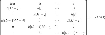
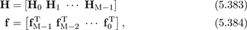
   2. We can express the FSE filter coefficients in the following matrix form:

      

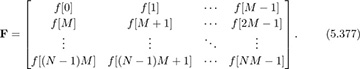
      We can interpret every (j + 1)^th column of F as a T-spaced subequalizer f_j[n] where j = 0, 2, ..., M −1. Similarly, we can express the FSE output, the channel coefficients, and the noise as T-spaced subsequences:

      

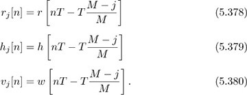
      Using these expressions, show that

      

   3. Now, express y_M [n] as a function of s[n], f_j[n], h_j[n], and υ_j[n]. This expression is known as the multichannel model of the FSE since the output is the sum of the symbols convolved with the T-spaced subequalizers and subsequences.

   4. Draw a block diagram of the multichannel model of the FSE based on part (c).

   5. Now consider a noise-free case. Given the channel matrix H_j given by

      

      we define

      

      where fj is the (j^th + 1) column of F. Perfect channel equalization can occur only if the solution to h = Cf, e = e_d lies in the column space of H, and the channel H has all linearly independent rows. What are the conditions on the length of the equalizer N given M_rx and L to ensure that the latter condition is met? Hint: What are the dimensions of the matrices/vectors?

   6. Given your answer in (e), consider the case of M = 1 (i.e., not using an FSE). Can perfect equalization be performed in this case?

10. Consider an order L-tap frequency-selective channel. After matched filtering, the received signal is

    

    where s[n] is the transmitted symbols, h[ℓ] is the channel coefficient, and υ[n] is AWGN. Suppose the received symbols corresponding to a known training sequence {1, −1, −1, 1} are {0.75 + j0.75, −0.75 − j0.25, −0.25 − j0.25, 0.25 + j0.75}. Note that this problem requires numerical solutions; that is, when you are asked to solve the least squares problems, the results must be specific numbers. MATLAB, LabVIEW, or MathScript in LabVIEW might be useful for solving the problem.

    1. Formulate the least squares estimator of in the matrix form. Do not solve it yet. Be explicit about your matrices and vectors, and list your assumptions (especially the assumption about the relationship between L and the length of the training sequence).

    2. Assuming L = 1, solve for the least squares channel estimate based on part (a).

    3. Assume we use a linear equalizer to remove the eff ects of the channel. Let be an FIR equalizer. Let n_d be the equalizer delay. Formulate the least squares estimator of given the channel estimate in part (b). Do not solve it yet.

    4. Determine the range of values of n_d.

    5. Determine the n_d that minimizes the squared error J_f[n_d] and solve for the least squares equalizer corresponding to this n_d. Also provide the value of the minimum squared error.

    6. With the same assumptions as in parts (a) through (e) and with the value of n_d found in part (e), formulate and solve for the direct least squares estimator of the equalizer’s coefficients . Also provide the value of the squared error.

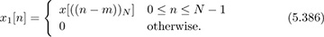
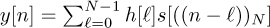
11. Prove the following two properties of the DFT:

    1. Let x[n] ↔ X[k] and x₁[n] ↔ X₁[k]. If X₁[k] = e^j2πkm/nX[k], we have

       

    2. Let y[n] ↔ Y [k], h[n] ↔ H[k] and s[n] ↔ S[k]. If Y [k] = H[k]S[k], we have .

12. Consider an OFDM system. Suppose that your buddy C.P. uses a cyclic postfix instead of a cyclic prefix. Thus

    

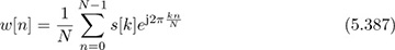
    for n = 0, 1, . . . , N + L_c where L_c is the length of the cyclic prefix. The values of w[n] for n < 0 and n > N + L_c are unknown. Let the received signal be

    

    1. Show that you can still recover with a cyclic postfix instead of a cyclic prefix.

    2. Draw a block diagram of the system.

    3. What are the differences between using a cyclic prefix and a cyclic postfix?

13. Consider an SC-FDE system with equivalent system . The length of the cyclic prefix is L_c. Prove that the cyclic prefix length should satisfy L_c ≥ L.

14. Consider an OFDM system with N = 256 subcarriers in 5MHz of bandwidth, with a carrier of f_c = 2GHz and a length L = 16 cyclic prefix. You can assume sinc pulse shaping.

    1. What is the subcarrier bandwidth?

    2. What is the length of the guard interval?

    3. Suppose you want to make the OFDM symbol periodic including the cyclic prefix. The length of the period will be 16. Which subcarriers do you need to zero in the OFDM symbol?

    4. What is the range of frequency offsets that you can correct using this approach?

15. Consider an OFDM system with N subcarriers.

    1. Derive a bound on the bit error probability for 4-QAM transmission. Your answer should depend on h[k], N_o, and d_min.

    2. Plot the error rate curves as a function of SNR for N = 1, 2, 4, assuming that h[0] = E_x, h[1] = E_x/2, h[2] = −jE_x/2, and h[3] = E_xe^−j2π/3/3.

16. How many pilot symbols are used in the OFDM symbols during normal data transmission (not the CEF) in IEEE 802.11a?

17. IEEE 802.11ad is a WLAN standard operating at 60GHz. It has much wider bandwidth than previous WLAN standards in lower-frequency bands. Four PHY formats are defined in IEEE 802.11ad, and one of them uses OFDM. The system uses a bandwidth of 1880MHz, with 512 subcarriers and a fixed 25% cyclic prefix. Now compute the following:

    1. What is the sample period duration assuming sampling at the Nyquist rate?

    2. What is the subcarrier spacing?

    3. What is the duration of the guard interval?

    4. What is the OFDM symbol period duration?

    5. In the standard among the 512 subcarriers, only 336 are used as data subcarriers. Assuming we use code rate 1/2 and QPSK modulation, compute the maximum data rate of the system.

18. Consider an OFDM communication system and a discrete-time channel with taps . Show mathematically why the cyclic prefix length L_c must satisfy L ≥ L_c.

19. In practice, we may want to use multiple antennas to improve the performance of the received signal. Suppose that the received signal for each antenna can be modeled as

    

    Essentially you have two observations of the same signal. Each is convolved by a different discrete-time channel.

    In this problem we determine the coefficients of a set of equalizers and such that

    

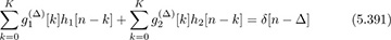
    where Δ is a design parameter.

    1. Suppose that you send training data . Formulate a least squares estimator for finding the estimated coefficients of the channel and .

    2. Formulate the least squares equalizer design problem given your channel estimate. Hint: You need a squared error. Do not solve it yet. Be explicit about your matrices and vectors.

    3. Solve for the least squares equalizer estimate using the formulation in part (b). You can use matrices in your answer. List your assumptions about dimensions and so forth.

    4. Draw a block diagram of a QAM receiver that includes this channel estimator and equalizer.

    5. Now formulate and solve the direct equalizer estimation problem. List your assumptions about dimensions and so forth.

    6. Draw a block diagram of a QAM receiver that includes this equalizer.

20. Consider a wireless communication system with a frame structure as illustrated in Figure 5.39. Training is interleaved around (potentially different) bursts of data. The same training sequence is repeated. This structure was proposed relatively recently and is used in the single-carrier mode in several 60GHz wireless communication standards.

    

    Figure 5.39 Frames with training data

    Let the training sequence be and the data symbols be {s[n]}. Just to make the problem concrete, suppose that

    

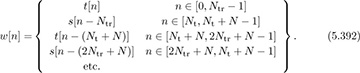
    Suppose that the channel is linear and time invariant. After matched filtering, synchronization, and sampling, the received signal is given by the usual relationship

    

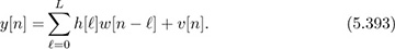
    Assume that N is much greater than N_tr, and that N_tr ≥ L.

    1. Consider the sequence . Show that there exists a cyclic prefix of length N_tr.

    2. Derive a single-carrier frequency-domain equalization structure that exploits the cyclic prefix we have created. Essentially, show how we can recover from {y[n]}.

    3. Draw a block diagram for the transmitter. You need to be as explicit as possible in indicating how the training sequence gets incorporated.

    4. Draw a block diagram for the receiver. Be careful.

    5. Suppose that we want to estimate the channel from the training sequence using the training on either side of the data. Derive the least squares channel estimator and determine the minimum value of N_tr required for this estimator to satisfy the conditions required by least squares.

    6. Can you use this same trick with OFDM, using training for the cyclic prefix? Explain why or why not.

21. Consider an OFDM communication system. Suppose that the system uses a bandwidth of 40MHz, 128 subcarriers, and a length 32 cyclic prefix. Suppose the carrier frequency is 5.785GHz.

    1. What is the sample period duration assuming sampling at the Nyquist rate?

    2. What is the OFDM symbol period duration?

    3. What is the subcarrier spacing?

    4. What is the duration of the guard interval?

    5. How much frequency offset can be corrected, in hertz, using the Schmidl-Cox method with all odd subcarriers zeroed, assuming only fine offset correction? Ignore the integer offset.

    6. Oscillators are specified in terms of their offset in parts per million. Determine how many parts per million of variation are tolerable given the frequency offset in part (e).

22. Consider an OFDM communication system with cyclic prefix of length L_c. The samples conveyed to the pulse-shaping filter are

    

    Recall that

    

    is the cyclic prefix. Suppose that the cyclic prefix is designed such that the channel order L satisfies L_c = 2L. In this problem, we use the cyclic prefix to perform carrier frequency offset estimation. Let the receive signal after match filtering, frame offset correction, and downsampling be written as

    

    1. Consider first a single OFDM symbol. Use the redundancy in the cyclic prefix to derive a carrier frequency offset estimator. Hint: Exploit the redundancy in the cyclic prefix but remember that L_c = 2L. You need to use the fact that the cyclic prefix is longer than the channel.

    2. What is the correction range of your estimator?

    3. Incorporate multiple OFDM symbols into your estimator. Does it work if the channel changes for different OFDM symbols?

23. Synchronization Using Repeated Training Sequences and Sign Flipping Consider the framing structure illustrated in Figure 5.40. This system uses a repetition of four training sequences. The goal of this problem is to explore the impact of multiple repeated training sequences on frame synchronization, frequency offset synchronization, and channel estimation.

    

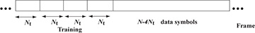
    Figure 5.40 A communication frame with four repeated training sequences followed by data symbols

    1. Suppose that you apply the frame synchronization, frequency offset estimation, and channel estimation algorithms using only two length N_tr training sequences. In other words, ignore the two additional repetitions of the training signal. Please comment on how frame synchronization, frequency offset estimation, and channel estimation work on the aforementioned packet structure.

    2. Now focus on frequency offset estimation. Treat the framing structure as a repetition of two length 2N_tr training signals. Present a correlation-based frequency offset estimator that uses two length 2N_tr training signals.

    3. Treat the framing structure as a repetition of four length N_tr training signals. Propose a frequency offset estimator that uses correlations of length N_tr and exploits all four training signals.

    4. What range of frequency offsets can be corrected in part (b) versus part (c)? Which is better in terms of accuracy versus range? Overall, which approach is better in terms of frame synchronization, frequency offset synchronization, and channel estimation? Please justify your answer.

    5. Suppose that we flip the sign of the third training sequence. Thus the training pattern becomes T, T, −T, T instead of T, T, T, T. Propose a frequency offset estimator that uses correlations of length N_tr and exploits all four training signals.

    6. What range of frequency offsets can be corrected in this case? From a frame synchronization perspective, what is the advantage of this algorithm versus the previoius algorithm you derived?

24. Synchronization in OFDM Systems Suppose that we would like to implement the frequency offset estimation algorithm. Suppose that our OFDM systems operate with N = 128 subcarriers in 2MHz of bandwidth, with a carrier of f_c = 1GHz and a length L = 16 cyclic prefix.

    1. What is the subcarrier bandwidth?

    2. We would like to design a training symbol that has the desirable periodic correlation properties that are useful in the discussed algorithm. What period should you choose and why? Be sure to consider the effect of the cyclic prefix.

    3. For the period you suggest in part (b), which subcarriers do you need to zero in the OFDM symbol?

    4. What is the range of frequency offsets that you can correct using this approach without requiring the modulo correction?

25. Consider the IEEE 802.11a standard. By thinking about the system design, provide plausible explanations for the following:

    1. Determine the amount of carrier frequency offset correction that can be obtained from the short training sequence.

    2. Determine the amount of carrier frequency offset correction that can be obtained from the long training sequence.

    3. Why do you suppose the long training sequence has a double-length guard interval followed by two repetitions?

    4. Why do you suppose that the training comes at the beginning instead of at the middle of the transmission as in the mobile cellular system GSM?

    5. Suppose that you use 10MHz instead of 20MHz in IEEE 802.11a. Would you rather change the DFT size or change the number of zero subcarriers?

26. Answer the following questions for problem 17:

    1. How much frequency offset (in Hertz) can be corrected using the Schmidl-Cox method with all odd subcarriers zeroed, assuming only fine offset correction? Ignore the integer offset.

    2. Oscillator frequency offsets are specified in parts per million (ppm). Determine how many parts per million of variation are tolerable given the result in part (a).

27. GMSK is an example of continuous-phase modulation (CPM). Its continuous-time baseband transmitted signal can be written as

    

    where a[n] is a sequence of BPSK symbols and ϕ(t) is the CPM pulse. For GSM, T = 6/1.625e6 ≈ 3.69µs.

    The BPSK symbol sequence a[n] is generated from a differentially binary (0 or 1) encoded data sequence d[n] where

    

    where ⊕ denotes modulo-2 addition. Let us denote the BPSK encoded data sequence as

    

    Then (5.398) can be rewritten in a simpler form as

    

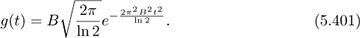
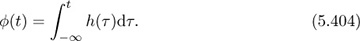
    Consider the Gaussian pulse response

    

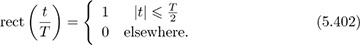
    Denote the rectangle function of duration T in the usual way as

    

    For GSM, BT = 0.3. This means that B = 81.25kHz. The B here is not the bandwidth of the signal; rather it is the 3dB bandwidth of the pulse g(t).

    The combined filter response is

    

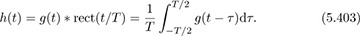
    Then the CPM pulse is given by

    

    Because of the choice of BT product, it is recognized that

    

    This means that the current GMSK symbol a[n] depends most strongly on the three previous symbols a[n − 1], a[n − 2], and a[n − 3].

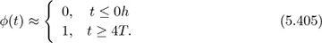
    Note that the phase output ϕ(t) depends on all previous bits d[n] because of the infinite integral. Consequently, the GSM modulator is initialized by the state give in Figure 5.41. The state is reinitialized for every transmitted burst.

    

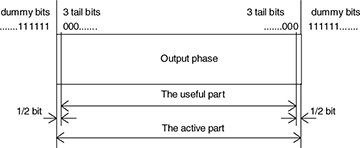
    Figure 5.41 GMSK is a modulation with memory. This figure based on [99] shows how each burst is assumed to be initialized.

    The classic references for linearization are [171, 173], based on the pioneering work on linearizing CPM signals in [187]. Here we summarize the linearization approach of [171, 173], which was used in [87] for the purpose of blind channel equalization of GMSK signals. We sketch the idea of the derivation from [87] here.

    1. Exploiting the observation in (5.405), argue that

       

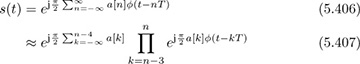
       for t ∈ [nT, (n+1)T). This makes the dependence of s(t) on the current symbol and past three symbols clearer.

    2. Explain how to obtain

       

    3. Using the fact that a[n] are BPSK modulated with values +1 or −1, and the even property of cosine and the odd property of sine, show that

       

    4. Now let

       

       Note that for any real number t = sgn(t) |t|. Now define

       

       It can be shown exploiting the symmetry of ϕ(t) that

       

       Substitute in for β to obtain

       

    5. Show that

       

       where

       

       and

       

       for t ∈ [0, 5T]. This is called the one-term approximation.

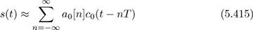
    6. Modify the typical transmit block diagram to implement the transmit waveform in (5.415).

    7. Modify the typical receiver block diagram to implement the receiver processing in a frequency-selective channel.

28. Plot the path loss for a distance from 1m to 200m for the following channel models and given parameters. The path loss should be plotted in decibels.

    1. Free space assuming G_t = G_r = 3dB, and λ = 0.1m

    2. Mean log distance using a 1m reference with free-space parameters as in part (a) with path-loss exponent β = 2

    3. Mean log distance using a 1m reference with free-space parameters as in part (a) with path-loss exponent β = 3

    4. Mean log distance using a 1m reference with free-space parameters as in part (a) with path-loss exponent β = 4

29. Plot the path loss at a distance of 1km for wavelengths from 10m to 0.01m for the following channel models and given parameters. The path loss should be plotted in decibels and the distance plotted on a log scale.

    1. Free space assuming G_t = G_r = 3dB

    2. Mean log distance using a 1m reference with free-space parameters as in part (a) with path-loss exponent β = 2

    3. Mean log distance using a 1m reference with free-space parameters as in part (a) with path-loss exponent β = 3

    4. Mean log distance using a 1m reference with free-space parameters as in part (a) with path-loss exponent β = 4

30. Consider the path loss for the log-distance model with shadowing for σ_shad = 8dB, η = 4, a reference distance of 1m with reference loss computed from free space, assuming G_r = G_r = 3dB, for a distance from 1m to 200m. Plot the mean path loss. For every value of d you plot, also plot the path loss for ten realizations assuming shadow fading. Explain what you observe. To resolve this issue, some path-loss models have a distance-dependent σ_shad.

31. Consider the LOS/NLOS path-loss model with P_los(d) = e^−d/200, free space for the LOS path loss, log distance without shadowing for the NLOS with β = 4, reference distance of 1m, G_t = G_r = 0dB, and λ = 0.1m. Plot the path loss in decibels for distances from 1 to 400m.

    1. Plot the LOS path loss.

    2. Plot the NLOS path loss.

    3. Plot the mean path loss.

    4. For each value of distance in your plot, generate ten realizations of the path loss and overlay them on your plot.

    5. Explain what happens as distances become larger.

32. Consider the path loss for the log-distance model assuming that β = 3, with reference distance 1m, G_t = G_r = 0dB and λ = 0.1m, and σ_shad = 6dB. The transmit power is P_tx = 10dBm. Generate your plots from 1 to 500m.

    1. Plot the received power based on the mean path-loss equation.

    2. Plot the probability that P_rx(d) < −110dBm.

    3. Determine the maximum value of d such that P_rx(d) > −110dBm 90% of the time.

33. Consider the LOS/NLOS path-loss model with P_los(d) = e^−d/200, free space for the LOS path loss, log distance without shadowing for the NLOS with β = 4, reference distance of 1m, G_t = G_r = 0dB, and λ = 0.1m. The transmit power is P_tx = 10dBm. Generate your plots from 1 to 500m.

    1. Plot the received power based on the mean path-loss equation.

    2. Plot the probability that P_rx(d) < −110dBm.

    3. Determine the maximum value of d such that P_rx(d) > −110dBm 90% of the time.

34. Consider the same setup as in the previous problem but now with shadowing on the NLOS component with σ_shad = 6dB. This problem requires some extra work to include the shadowing in the NLOS part.

    1. Plot a realization of the received path loss here. Do not forget about the shadowing.

    2. Plot the probability that P_rx(d) < −110dBm.

    3. Determine the maximum value of d such that P_rx(d) > −110dBm 90% of the time.

35. Consider a simple cellular system. Seven base stations are located in a hexagonal cluster, with one in the center and six surrounding. Specifically, there is a base station at the origin and six base stations located 400m away at 0°, 60°, 120°, and so on. Consider the path loss for the log-distance model assuming that β = 4, with reference distance 1m, G_t = G_r = 0dB, and λ = 0.1m. You can use 290K and a bandwidth of B = 10MHz to compute the thermal noise power as kTB. The transmit power is P_tx = 40dBm.

    1. Plot the SINR for a user moving along the 0° line from a distance of 1m from the base station to 300m. Explain what happens in this curve.

    2. Plot the mean SINR for a user from a distance of 1m from the base station to 300m. Use Monte Carlo simulations. For every distance, generate 100 user locations randomly on a circle of radius d and average the results. How does this compare with the previous curve?

36. Link Budget Calculations In this problem you will compute the acceptable transmission range by going through a link budget calculation. You will need the fact that noise variance is kTB where k is Boltzmann’s constant (i.e., k = 1.381 × 10⁻²³W/Hz/K), T is the effective temperature in kelvins (you can use T = 300K), and B is the signal bandwidth. Suppose that field measurements were made inside a building and that subsequent processing revealed that the data fit the log-normal model. The path-loss exponent was found to be n = 4. Suppose that the transmit power is 50mW, 10mW is measured at a reference distance d₀ = 1m from the transmitter, and σ = 8dB for the log-normal path-loss model. The desired signal bandwidth is 1MHz, which is found to be sufficiently less than the coherence bandwidth; thus the channel is well modeled by the Rayleigh fading channels. Use 4-QAM modulation.

    1. Calculate the noise power in decibels referenced to 1 milliwatt (dBm).

    2. Determine the SNR required for the Gaussian channel to have a symbol error rate of 10⁻². Using this value and the noise power, determine the minimum received signal power required for at least 10⁻² operation. Let this be P_min (in decibels as usual).

    3. Determine the largest distance such that the received power is above P_min.

    4. Determine the small-scale link margin L_Rayleigh for the flat Rayleigh fading channel. The fade margin is the difference between the SNR required for the Rayleigh case and the SNR required for the Gaussian case. Let P_Rayleigh = L_Rayleigh + P_min.

    5. Determine the large-scale link margin for the log-normal channel with a 90% outage. In other words, find the received power P_large-scale required such that P_large-scale is greater than P_Rayleigh 90% of the time.

    6. Using P_large-scale, determine the largest acceptable distance in meters that the system can support.

    7. Ignoring the effect of small-scale fading, what is the largest acceptable distance in meters that the system can support?

    8. Describe the potential impact of diversity on the range of the system.

37. Suppose that field measurements were made inside a building and that subsequent processing revealed that the data fit the path-loss model with shadowing. The path-loss exponent was found to be n = 3.5. If 1mW was measured at d₀ = 1m from the transmitter and at a distance of d₀ = 10m, 10% of the measurements were stronger than −25dBm, find the standard deviation σ_shad for the log-normal model.

38. Through real measurement, the following three received power measurements were obtained at distances of 100m, 400m, and 1.6km from a transmitter:

    

    Click to view larger image

    1. Suppose that the path loss follows the log-distance model, without shadowing, with reference distance d₀ = 100m. Use least squares to estimate the path-loss exponent.

    2. Suppose that the noise power is −90dBm and the target SNR is 10dB. What is the minimum received signal power required, also known as the receiver sensitivity?

    3. Using the value calculated in part (b), what is the approximate acceptable largest distance in kilometers that the system can support?

39. Classify the following as slow or fast and frequency selective or frequency flat. Justify your answers. In some cases you will have to argue why your answer is correct by making reasonable assumptions based on the application. Assume that the system occupies the full bandwidth listed.

    1. A cellular system with carrier frequency of 2GHz, bandwidth of 1.25MHz, that provides service to high-speed trains. The RMS delay spread is 2µs.

    2. A vehicle-to-vehicle communication system with carrier frequency of 800MHz and bandwidth of 100kHz. The RMS delay spread is 20ns.

    3. A 5G communication system with carrier frequency of 3.7GHz and bandwidth of 200MHz.

    4. A 60GHz wireless personal area network with a bandwidth of 2GHz and an RMS delay spread of 40ns. The main application is high-speed multimedia delivery.

    5. Police-band radio. Vehicles move at upwards of 100mph and communicate with a base station. The bandwidth is 50kHz at 900MHz carrier.

40. Consider a wireless communication system with a frequency carrier of f_c = 1.9GHz and a bandwidth of B = 5MHz. The power delay profile shows the presence of three strong paths and is plotted in Figure 5.42.

    

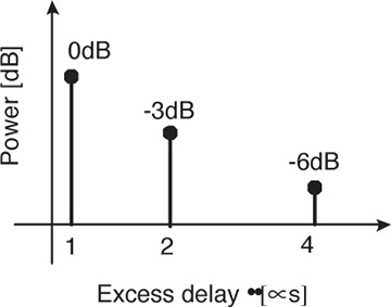
    Figure 5.42 The power delay profile of a three-path channel

    1. Compute the RMS delay spread.

    2. Consider a single-carrier wireless system. Classify the system as frequency flat or frequency selective and slow or fast. Assume the system provides service to vehicle-to-vehicle communication at the speed of υ = 120km/h and not packet transmission but symbol transmission. You should use the stricter relationship between coherence time T_coh and maximum Doppler frequency f_m by .

    3. Consider an OFDM system with IFFT/FFT size of N = 1024. What is the maximum-length cyclic prefix needed to allow for efficient equalization in the frequency domain with OFDM?

    4. For the specified OFDM system, which also provides services to vehicle-to-vehicle communication at urban speeds of 30mph, is the channel slow or fast fading? Justify your answer.

41. Suppose that R_delay(τ) = 1 for τ ∈ [0, 20µs] and is zero otherwise.

    1. Compute the RMS delay spread.

    2. Compute the spaced-frequency correlation function S_delay(Δ_lag).

    3. Determine if the channel is frequency selective or frequency flat for a signal with bandwidth B = 1MHz.

    4. Find the largest value of bandwidth such that the channel can be assumed to be frequency flat.

42. Suppose that for τ ∈ [0, 20µs].

    1. Compute the RMS delay spread.

    2. Compute the spaced-frequency correlation function S_delay(Δ_lag).

    3. Determine if the channel is frequency selective or frequency flat for a signal with bandwidth B = 1MHz.

    4. Find the largest value of bandwidth such that the channel can be assumed to be frequency flat.

43. Sketch the design of an OFDM system with 80MHz channels, supporting pedestrian speeds of 3km/h, an RMS delay spread of 8µs, operating at f_c = 800MHz. Explain how you would design the preamble to permit synchronization and channel estimation and how you would pick the parameters such as the number of subcarriers and the cyclic prefix. Justify your choice of parameters and explain how you deal with mobility, delay spread, and how much frequency offset you can tolerate. You do not need to do any simulation for this problem; rather make calculations as required and then justify your answers.

44. Sketch the design of an SC-FDE system with 2GHz channels, supporting pedestrian speeds of 3km/h, and an RMS delay spread of 50ns, operating at f_c = 64GHz. Explain how you would design the preamble to permit synchronization and channel estimation and how you would pick the parameters. Justify your choice of parameters and explain how you deal with mobility, delay spread, and how much frequency offset you can tolerate. You do not need to do any simulation for this problem; rather make calculations as required and then justify your answers.

45. Consider an OFDM system with a bandwidth of W = 10MHz. The power delay profile estimates the RMS delay spread to be σ_RMS,delay = 5µs. Possible IFFT/FFT sizes for the system are N = {128, 256, 512, 1024, 2048}. Possible cyclic prefix sizes (in terms of fractions of N) are {1/4, 1/8, 1/16, 1/32}.

    1. What combination of FFT and cyclic prefix sizes provides the minimum amount of overhead?

    2. Calculate the fraction of loss due to this overhead.

    3. What might be some issues associated with minimizing the amount of overhead in this system?

46. Compute the maximum Doppler shift for the following sets of parameters:

    1. 40MHz of bandwidth, carrier of 2.4GHz, and supporting 3km/h speeds

    2. 2GHz of bandwidth, carrier of 64GHz, and supporting 3km/h speeds

    3. 20MHz of bandwidth, carrier of 2.1GHz, and supporting 300km/h speeds

47. In fixed wireless systems, the Clarke-Jakes spectrum may not be appropriate. A better model is the Bell Doppler spectrum where 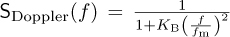has been found to fit to data [363] where K_B is a constant so that ∫_fS_Doppler(f)df = 1. In this case, the maximum Doppler shift is determined from the Doppler due to moving objects in the environment.

    1. Determine K_B for a maximum velocity of 160km/h and a carrier frequency of 1.9GHz.

    2. Determine the RMS Doppler spread.

    3. Is a signal with bandwidth of B = 20MHz and blocks of length 1000 symbols well modeled as time invariant?

48. Look up the basic parameters of the GSM cellular system. Consider a dual-band phone that supports f_c = 900MHz and f_c = 1.8GHz. What is the maximum velocity that can be supported on each carrier frequency so that the channel is sufficiently constant during a burst period? Explain your work and list your assumptions.

49. Look up the basic parameters of an IEEE 802.11a system. What is the maximum amount of delay spread that can be tolerated by an IEEE 802.11a system? Suppose that you are in a square room and that the access point is located in the middle of the room. Consider single reflections. How big does the room need to be to give this maximum amount of channel delay?

50. Consider 4-QAM transmission. Plot the following for error rates of 1 to 10⁻⁵ and SNRs of 0dB to 30dB. This means that for higher SNRs do not plot values of the error rate below 10⁻⁵.

    • Gaussian channel, exact expression

    • Gaussian channel, exact expression, neglecting the quadratic term

    • Gaussian channel, exact expression, neglecting the quadratic term and using a Chernoff upper bound on the Q-function

    • Rayleigh fading channel, Chernoff upper bound on the Q-function

51. Computer In this problem, you will create a flat-fading channel simulator function. The input to your function is x(nT/M_tx), the sampled pulse-amplitude modulated sequence sampled at T/M_tx where M_tx is the oversampling factor. The output of your function is r(nT/M_rx), which is the sampled receive pulse-amplitude modulated signal (5.7). The parameters of your function should be the channel h (which does not include ), the delay τ_d, M_tx, M_rx, and the frequency offset . Essentially, you need to determine the discrete-time equivalent channel, convolve it with x(nT/M_tx), resample, incorporate frequency offset, add AWGN, and resample to produce r(nT/M_rx). Be sure that the noise is added correctly so it is correlated. Design some tests and demonstrate that your code works correctly.

52. Computer In this problem, you will create a symbol synchronization function. The input is y(nT/M_rx), which is the matched filtered receive pulse-amplitude modulated signal, M_rx the receiver oversampling factor, and the block length for averaging. You should implement both versions of the MOE algorithm. Demonstrate that your code works. Simulate x(t) obtained from 4-QAM constellations with 100 symbols and raised cosine pulse shaping with α = 0.25. Pass your sampled signal with M_tx ≥ 2 through your channel simulator to produce the sampled output with M_rx samples per symbol. Using a Monte Carlo simulation, with an offset of τ_d = T/3 and h = 0.3e^jπ/3, perform 100 trials of estimating the symbol timing with each symbol synchronization algorithm for SNRs from 0dB to 10dB. Which one gives the best performance? Plot the received signal after correction; that is, plot for the entire frame with real on the x-axis and imaginary on the y-axis for 0dB and 10dB SNR. This should give a rotated set of 4-QAM constellation symbols. Explain your results.

53. Computer In this problem, you will implement the transmitter and receiver for a flat-fading channel. The communication system has a training sequence of length 32 that is composed of length 8 Golay sequences and its complementary pairs as [a₈, b₈, a₈, b₈]. The training sequence is followed by 100 M-QAM symbols. No symbols are sent before or after this packet. Suppose that M_rx = 8, τ_d = 4T +T/3, and h = e^jπ/3. There is no frequency offset. Generate the matched filtered receive signal. Pass it through your symbol timing synchronizer and correct for the timing error. Then perform the following:

    1. Develop a frame synchronization algorithm using the given training sequence. Demonstrate the performance of your algorithm by performing 100 Monte Carlo simulations for a range of SNR values from 0dB to 10dB. Count the number of frame synchronization errors as a function of SNR.

    2. After correction for frame synchronization error, estimate the channel. Plot the estimation error averaged over all the Monte Carlo trials as a function of SNR.

    3. Compute the probability of symbol error. Perform enough Monte Carlo trials to estimate the symbol error reliably to 10⁻⁴.

54. Computer Consider the same setup as in the previous problem but now with a frequency offset of = 0.03. Devise and implement a frequency offset correction algorithm.

    1. Assuming no delay in the channel, demonstrate the performance of your algorithm by performing 100 Monte Carlo simulations for a range of SNR values from 0dB to 10dB. Plot the average frequency offset estimation error.

    2. After correction for frequency synchronization error, estimate the channel. Plot the estimation error averaged over all the Monte Carlo trials as a function of SNR.

    3. Perform enough Monte Carlo trials to estimate the symbol error reliably to 10⁻⁴.

    4. Repeat each of the preceding tasks by now including frame synchronization and symbol timing with τ_d as developed in the previous problem. Explain your results.

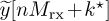
55. Computer In this problem, you will create a multipath channel simulator function where the complex baseband equivalent channel has the form

    

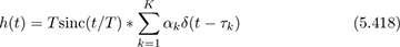
    and the channel has multiple taps, each consisting of complex amplitude α_k and delay τ_k. The input to your function is x(nT/M_tx), the sampled pulse-amplitude modulated sequence sampled at T/M_tx where M_tx is the oversampling factor. The output of your function is r(nT/M_rx), which is sampled from

    

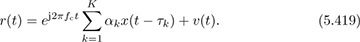
    Your simulator should include the channel parameters M_tx, M_rx, and the frequency offset . Check that your code works correctly by comparing it with the flat-fading channel simulator. Design some other test cases and demonstrate that your code works.