The Art of Computer Programming, Volume 3: Combinatorial Properties of Permutations

This chapter is from the book 

*5.1. Combinatorial Properties of Permutations

A permutation of a finite set is an arrangement of its elements into a row. Permutations are of special importance in the study of sorting algorithms, since they represent the unsorted input data. In order to study the efficiency of different sorting methods, we will want to be able to count the number of permutations that cause a certain step of a sorting procedure to be executed a certain number of times.

We have, of course, met permutations frequently in previous chapters. For example, in Section 1.2.5 we discussed two basic theoretical methods of constructing the n! permutations of n objects; in Section 1.3.3 we analyzed some algorithms dealing with the cycle structure and multiplicative properties of permutations; in Section 3.3.2 we studied their “runs up” and “runs down.” The purpose of the present section is to study several other properties of permutations, and to consider the general case where equal elements are allowed to appear. In the course of this study we will learn a good deal about combinatorial mathematics.

The properties of permutations are sufficiently pleasing to be interesting in their own right, and it is convenient to develop them systematically in one place instead of scattering the material throughout this chapter. But readers who are not mathematically inclined and readers who are anxious to dive right into sorting techniques are advised to go on to Section 5.2 immediately, since the present section actually has little direct connection to sorting.

*5.1.1. Inversions

Let a₁ a₂ . . . a_n be a permutation of the set {1, 2, . . ., n}. If i < j and a_i > a_j, the pair (a_i, a_j) is called an inversion of the permutation; for example, the permutation 3 1 4 2 has three inversions: (3, 1), (3, 2), and (4, 2). Each inversion is a pair of elements that is out of sort, so the only permutation with no inversions is the sorted permutation 1 2 . . . n. This connection with sorting is the chief reason why we will be so interested in inversions, although we have already used the concept to analyze a dynamic storage allocation algorithm (see exercise 2.2.2–9).

The concept of inversions was introduced by G. Cramer in 1750 [Intr. à l’Analyse des Lignes Courbes Algébriques (Geneva: 1750), 657–659; see Thomas Muir, Theory of Determinants 1 (1906), 11–14], in connection with his famous rule for solving linear equations. In essence, Cramer defined the determinant of an n × n matrix in the following way:

summed over all permutations a₁ a₂ . . . a_n of {1, 2, . . ., n}, where inv(a₁ a₂ . . . a_n) is the number of inversions of the permutation.

The inversion table b₁ b₂ . . . b_n of the permutation a₁ a₂ . . . a_n is obtained by letting b_j be the number of elements to the left of j that are greater than j. In other words, b_j is the number of inversions whose second component is j. It follows, for example, that the permutation

Equation (1)

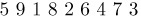
has the inversion table

Equation (2)

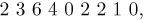
since 5 and 9 are to the left of 1; 5, 9, 8 are to the left of 2; etc. This permutation has 20 inversions in all. By definition the numbers b_j will always satisfy

Equation (3)

Perhaps the most important fact about inversions is the simple observation that an inversion table uniquely determines the corresponding permutation. We can go back from any inversion table b₁ b₂ . . . b_n satisfying (3) to the unique permutation that produces it, by successively determining the relative placement of the elements n, n−1, . . . , 1 (in this order). For example, we can construct the permutation corresponding to (2) as follows: Write down the number 9; then place 8 after 9, since b₈ = 1. Similarly, put 7 after both 8 and 9, since b₇ = 2. Then 6 must follow two of the numbers already written down, because b₆ = 2; the partial result so far is therefore

• 9 8 6 7.

Continue by placing 5 at the left, since b₅ = 0; put 4 after four of the numbers; and put 3 after six numbers (namely at the extreme right), giving

• 5 9 8 6 4 7 3.

The insertion of 2 and 1 in an analogous way yields (1).

This correspondence is important because we can often translate a problem stated in terms of permutations into an equivalent problem stated in terms of inversion tables, and the latter problem may be easier to solve. For example, consider the simplest question of all: How many permutations of {1, 2, . . ., n} are possible? The answer must be the number of possible inversion tables, and they are easily enumerated since there are n choices for b₁, independently n−1 choices for b₂, . . ., 1 choice for b_n, making n(n−1) . . . 1 = n! choices in all. Inversions are easy to count, because the b’s are completely independent of each other, while the a’s must be mutually distinct.

In Section 1.2.10 we analyzed the number of local maxima that occur when a permutation is read from right to left; in other words, we counted how many elements are larger than any of their successors. (The right-to-left maxima in (1), for example, are 3, 7, 8, and 9.) This is the number of j such that b_j has its maximum value, n − j. Since b₁ will equal n − 1 with probability 1/n, and (independently) b₂ will be equal to n − 2 with probability 1/(n − 1), etc., it is clear by consideration of the inversions that the average number of right-to-left maxima is

The corresponding generating function is also easily derived in a similar way.

If we interchange two adjacent elements of a permutation, it is easy to see that the total number of inversions will increase or decrease by unity. Figure 1 shows the 24 permutations of {1, 2, 3, 4}, with lines joining permutations that differ by an interchange of adjacent elements; following any line downward inverts exactly one new pair. Hence the number of inversions of a permutation π is the length of a downward path from 1234 to π in Fig. 1; all such paths must have the same length.

Incidentally, the diagram in Fig. 1 may be viewed as a three-dimensional solid, the “truncated octahedron,” which has 8 hexagonal faces and 6 square faces. This is one of the classical uniform polyhedra attributed to Archimedes (see exercise 10).

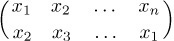
The reader should not confuse inversions of a permutation with the inverse of a permutation. Recall that we can write a permutation in two-line form

Equation (4)

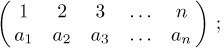
the inverse of this permutation is the permutation obtained by interchanging the two rows and then sorting the columns into increasing order of the new top row:

Equation (5)

For example, the inverse of 5 9 1 8 2 6 4 7 3 is 3 5 9 7 1 6 8 4 2, since

Another way to define the inverse is to say that if and only if a_k = j.

The inverse of a permutation was first defined by H. A. Rothe [in Sammlung combinatorisch-analytischer Abhandlungen, edited by C. F. Hindenburg, 2 (Leipzig: 1800), 263–305], who noticed an interesting connection between inverses and inversions: The inverse of a permutation has exactly as many inversions as the permutation itself. Rothe’s proof of this fact was not the simplest possible one, but it is instructive and quite pretty nevertheless. We construct an n × n chessboard having a dot in column j of row i whenever a_i = j. Then we put ×’s in all squares that have dots lying both below (in the same column) and to their right (in the same row). For example, the diagram for 5 9 1 8 2 6 4 7 3 is

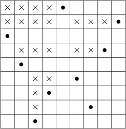
The number of ×’s is the number of inversions, since it is easy to see that b_j is the number of ×’s in column j. Now if we transpose the diagram—interchanging rows and columns — we get the diagram corresponding to the inverse of the original permutation. Hence the number of ×’s (the number of inversions) is the same in both cases. Rothe used this fact to prove that the determinant of a matrix is unchanged when the matrix is transposed.

The analysis of several sorting algorithms involves the knowledge of how many permutations of n elements have exactly k inversions. Let us denote that number by I_n(k); Table 1 lists the first few values of this function.

By considering the inversion table b₁ b₂ . . . b_n, it is obvious that I_n(0) = 1, I_n(1) = n − 1, and there is a symmetry property

Equation (6)

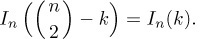
Table 1 Permutations with k Inversions

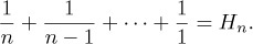
Furthermore, since each of the b’s can be chosen independently of the others, it is not difficult to see that the generating function

Equation (7)

satisfies G_n(z) = (1 + z + · · · + z^{n− 1})G_n−1(z); hence it has the comparatively simple form noticed by O. Rodrigues [J. de Math. 4 (1839), 236–240]:

Equation (8)

From this generating function, we can easily extend Table 1, and we can verify that the numbers below the zigzag line in that table satisfy

Equation (9)

(This relation does not hold above the zigzag line.) A more complicated argument (see exercise 14) shows that, in fact, we have the formulas

in general, the formula for I_n(k) contains about 1.6 terms:

Equation (10)

where u_j = (3j² − j)/2 is a so-called “pentagonal number.”

If we divide G_n(z) by n! we get the generating function g_n(z) for the probability distribution of the number of inversions in a random permutation of n elements. This is the product

Equation (11)

where h_k(z) = (1 + z + · · · + z^k−1)/k is the generating function for the uniform distribution of a random nonnegative integer less than k. It follows that

Equation (12)

Equation (13)

So the average number of inversions is rather large, about n²; the standard deviation is also rather large, about n^3/2.

A remarkable discovery about the distribution of inversions was made by P. A. MacMahon [Amer. J. Math. 35 (1913), 281–322]. Let us define the index of the permutation a₁ a₂ . . . a_n as the sum of all subscripts j such that a_j > a_j+1, 1 ≤ j < n. For example, the index of 5 9 1 8 2 6 4 7 3 is 2 + 4 + 6 + 8 = 20. By coincidence the index is the same as the number of inversions in this case. If we list the 24 permutations of {1, 2, 3, 4}, namely

we see that the number of permutations having a given index, k, is the same as the number having k inversions.

At first this fact might appear to be almost obvious, but further scrutiny makes it very mysterious. MacMahon gave an ingenious indirect proof, as follows: Let ind(a₁ a₂ . . . a_n) be the index of the permutation a₁ a₂ . . . a_n, and let

Equation (14)

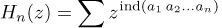
be the corresponding generating function; the sum in (14) is over all permutations of {1, 2, . . ., n}. We wish to show that H_n(z) = G_n(z). For this purpose we will define a one-to-one correspondence between arbitrary n-tuples (q₁, q₂, . . ., q_n) of nonnegative integers, on the one hand, and ordered pairs of n-tuples

((a₁, a₂, . . ., a_n), (p₁, p₂, . . ., p_n))

on the other hand, where a₁ a₂ . . . a_n is a permutation of the indices {1, 2, . . ., n} and p₁ ≥ p₂ ≥ · · · ≥ p_n ≥ 0. This correspondence will satisfy the condition

Equation (15)

The generating function ∑z^{q₁+q₂+···+q_n}, summed over all n-tuples of nonnegative integers (q₁, q₂, . . ., q_n), is Q_n(z) = 1/(1 − z)ⁿ; and the generating function ∑z^{p₁+p₂+···+p_n}, summed over all n-tuples of integers (p₁, p₂, . . ., p_n) such that p₁ ≥ p₂ ≥ · · · ≥ p_n ≥ 0, is

Equation (16)

as shown in exercise 15. In view of (15), the one-to-one correspondence we are about to establish will prove that Q_n(z) = H_n(z)P_n(z), that is,

Equation (17)

But Q_n(z)/P_n(z) is G_n(z), by (8).

The desired correspondence is defined by a simple sorting procedure: Any n-tuple (q₁, q₂, . . ., q_n) can be rearranged into nonincreasing order q_a1 ≥ q_a2 ≥ · · · ≥ q_an in a stable manner, where a₁ a₂ . . . a_n is a permutation such that q_aj = q_aj+1 implies a_j < a_j+1. We set (p₁, p₂, . . ., p_n) = (q_a1, q_a2, . . ., q_an) and then, for 1 ≤ j < n, subtract 1 from each of p₁, . . ., p_j for each j such that a_j > a_j+1. We still have p₁ ≥ p₂ ≥ · · · ≥ p_n, because p_j was strictly greater than p_j+1 whenever a_j > a_j+1. The resulting pair ((a₁, a₂, . . ., a_n), (p₁, p₂, . . ., p_n)) satisfies (15), because the total reduction of the p’s is ind(a₁ a₂ . . . a_n). For example, if n = 9 and (q₁, . . ., q₉) = (3, 1, 4, 1, 5, 9, 2, 6, 5), we find a₁ . . . a₉ = 6 8 5 9 3 1 7 2 4 and (p₁, . . ., p₉) = (5, 2, 2, 2, 2, 2, 1, 1, 1).

Conversely, we can easily go back to (q₁, q₂, . . ., q_n) when a₁ a₂ . . . a_n and (p₁, p₂, . . ., p_n) are given. (See exercise 17.) So the desired correspondence has been established, and MacMahon’s index theorem has been proved.

D. Foata and M. P. Schützenberger discovered a surprising extension of MacMahon’s theorem, about 65 years after MacMahon’s original publication: The number of permutations of n elements that have k inversions and index l is the same as the number that have l inversions and index k. In fact, Foata and Schützenberger found a simple one-to-one correspondence between permutations of the first kind and permutations of the second (see exercise 25).

Exercises

• 1. [10] What is the inversion table for the permutation 2 7 1 8 4 5 9 3 6? What permutation has the inversion table 5 0 1 2 1 2 0 0?

• 2. [M20] In the classical problem of Josephus (exercise 1.3.2–22), n men are initially arranged in a circle; the mth man is executed, the circle closes, and every mth man is repeatedly eliminated until all are dead. The resulting execution order is a permutation of {1, 2, . . ., n}. For example, when n = 8 and m = 4 the order is 5 4 6 1 3 8 7 2 (man 1 is 5th out, etc.); the inversion table corresponding to this permutation is 3 6 3 1 0 0 1 0.

  Give a simple recurrence relation for the elements b₁ b₂ . . . b_n of the inversion table in the general Josephus problem for n men, when every mth man is executed.

• 3. [18] If the permutation a₁ a₂ . . . a_n corresponds to the inversion table b₁ b₂ . . . b_n, what is the permutation ā₁ ā₂ . . . ā_n that corresponds to the inversion table

  • (n − 1 − b₁)(n − 2 − b₂) . . . (0 − b_n) ?
• ▸ 4. [20] Design an algorithm suitable for computer implementation that constructs the permutation a₁ a₂ . . . a_n corresponding to a given inversion table b₁ b₂ . . . b_n satisfying (3). [Hint: Consider a linked-memory technique.]
• 5. [35] The algorithm of exercise 4 requires an execution time roughly proportional to n + b₁ + · · · + b_n on typical computers, and this is Θ(n²) on the average. Is there an algorithm whose worst-case running time is substantially better than order n²?
• ▸ 6. [26] Design an algorithm that computes the inversion table b₁ b₂ . . . b_n corresponding to a given permutation a₁ a₂ . . . a_n of {1, 2, . . ., n}, where the running time is essentially proportional to n log n on typical computers.

• 7. [20] Several other kinds of inversion tables can be defined, corresponding to a given permutation a₁ a₂ . . . a_n of {1, 2, . . ., n}, besides the particular table b₁ b₂ . . . b_n defined in the text; in this exercise we will consider three other types of inversion tables that arise in applications.

  Let c_j be the number of inversions whose first component is j, that is, the number of elements to the right of j that are less than j. [Corresponding to (1) we have the table 0 0 0 1 4 2 1 5 7; clearly 0 ≤ c_j < j.] Let B_j = b_aj and C_j = c_aj.

  Show that 0 ≤ B_j < j and 0 ≤ C_j ≤ n − j, for 1 ≤ j ≤ n; furthermore show that the permutation a₁ a₂ . . . a_n can be determined uniquely when either c₁ c₂ . . . c_n or B₁ B₂ . . . B_n or C₁ C₂ . . . C_n is given.

• 8. [M24] Continuing the notation of exercise 7, let be the inverse of the permutation a₁ a₂ . . . a_n, and let the corresponding inversion tables be , , , and . Find as many interesting relations as you can between the numbers .
• ▸ 9. [M21] Prove that, in the notation of exercise 7, the permutation a₁ a₂ . . . a_n is an involution (that is, its own inverse) if and only if b_j = C_j for 1 ≤ j ≤ n.
• 10. [HM20] Consider Fig. 1 as a polyhedron in three dimensions. What is the diameter of the truncated octahedron (the distance between vertex 1234 and vertex 4321), if all of its edges have unit length?
• 11. [M25] If π = a₁ a₂ . . . a_n is a permutation of {1, 2, . . ., n}, let

  E(π) = {(a_i, a_j) | i < j, a_i > a_j}

  be the set of its inversions, and let

  Ē(π) = {(a_i, a_j) | i > j, a_i > a_j}

  be the non-inversions.

  1. Prove that E(π) and Ē(π) are transitive. (A set S of ordered pairs is called transitive if (a, c) is in S whenever both (a, b) and (b, c) are in S.)
  2. Conversely, let E be any transitive subset of T = {(x, y) | 1 ≤ y < x ≤ n} whose complement Ē = T \ E is also transitive. Prove that there exists a permutation π such that E(π) = E.
• 12. [M28] Continuing the notation of the previous exercise, prove that if π₁ and π₂ are permutations and if E is the smallest transitive set containing E(π₁) ∪ E(π₂), then Ē is transitive. [Hence, if we say π₁ is “above” π₂ whenever E(π₁) ⊆ E(π₂), a lattice of permutations is defined; there is a unique “lowest” permutation “above” two given permutations. Figure 1 is the lattice diagram when n = 4.]
• 13. [M23] It is well known that half of the terms in the expansion of a determinant have a plus sign, and half have a minus sign. In other words, there are just as many permutations with an even number of inversions as with an odd number, when n ≥ 2. Show that, in general, the number of permutations having a number of inversions congruent to t modulo m is n!/m, regardless of the integer t, whenever n ≥ m.

• 14. [M24] (F. Franklin.) A partition of n into k distinct parts is a representation n = p₁ + p₂ + · · · + p_k, where p₁ > p₂ > · · · > p_k > 0. For example, the partitions of 7 into distinct parts are 7, 6 + 1, 5 + 2, 4 + 3, 4 + 2 + 1. Let f_k(n) be the number of partitions of n into k distinct parts; prove that ∑_k (−1)^kf_k(n) = 0, unless n has the form (3j² ± j)/2, for some nonnegative integer j; in the latter case the sum is (−1)^j. For example, when n = 7 the sum is − 1 + 3 − 1 = 1, and 7 = (3 · 2² + 2)/2. [Hint: Represent a partition as an array of dots, putting p_i dots in the ith row, for 1 ≤ i ≤ k. Find the smallest j such that p_j+1 < p_j − 1, and encircle the rightmost dots in the first j rows. If j < p_k, these j dots can usually be removed, tilted 45°, and placed as a new (k+1)st row. On the other hand if j ≥ p_k, the kth row of dots can usually be removed, tilted 45°, and placed to the right of the circled dots. (See Fig. 2.) This process pairs off partitions having an odd number of rows with partitions having an even number of rows, in most cases, so only unpaired partitions must be considered in the sum.]

  

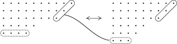
  Fig. 2. Franklin’s correspondence between partitions with distinct parts.

  Note: As a consequence, we obtain Euler’s formula

  

  Click to view larger image

  The generating function for ordinary partitions (whose parts are not necessarily distinct) is ∑p(n)zⁿ = 1/(1 − z)(1 − z²)(1 − z³) . . .; hence we obtain a nonobvious recurrence relation for the partition numbers,

  p(n) = p(n − 1) + p(n − 2) − p(n − 5) − p(n − 7) + p(n − 12) + p(n − 15) − · · · .

• 15. [M23] Prove that (16) is the generating function for partitions into at most n parts; that is, prove that the coefficient of z^m in 1/(1 − z)(1 − z²) . . . (1 − zⁿ) is the number of ways to write m = p₁ + p₂ + · · · + p_n with p₁ ≥ p₂ ≥ · · · ≥ p_n ≥ 0. [Hint: Drawing dots as in exercise 14, show that there is a one-to-one correspondence between n-tuples (p₁, p₂, . . ., p_n) such that p₁ ≥ p₂ ≥ · · · ≥ p_n ≥ 0 and sequences (P₁, P₂, P₃, . . .) such that n ≥ P₁ ≥ P₂ ≥ P₃ ≥ · · · ≥ 0, with the property that p₁ + p₂ + · · · + p_n = P₁ + P₂ + P₃ + · · · . In other words, partitions into at most n parts correspond to partitions into parts not exceeding n.]

• 16. [M25] (L. Euler.) Prove the following identities by interpreting both sides of the equations in terms of partitions:

  

  Click to view larger image

• 17. [20] In MacMahon’s correspondence defined at the end of this section, what are the 24 quadruples (q₁, q₂, q₃, q₄) for which (p₁, p₂, p₃, p₄) = (0, 0, 0, 0)?
• 18. [M30] (T. Hibbard, CACM 6 (1963), 210.) Let n > 0, and assume that a sequence of 2ⁿ n-bit integers X₀, . . ., X_2ⁿ−1 has been generated at random, where each bit of each number is independently equal to 1 with probability p. Consider the sequence X₀ ⊕ 0, X₁ ⊕ 1, . . ., X₂n˒1 ⊕ (2ⁿ − 1), where ⊕ denotes the “exclusive or” operation on the binary representations. Thus if p = 0, the sequence is 0, 1, . . . , 2ⁿ −1, and if p = 1 it is 2ⁿ −1, . . . , 1, 0; and when p = , each element of the sequence is a random integer between 0 and 2ⁿ − 1. For general p this is a useful way to generate a sequence of random integers with a biased number of inversions, although the distribution of the elements of the sequence taken as a whole is uniform in the sense that each n-bit integer has the same distribution. What is the average number of inversions in such a sequence, as a function of the probability p?
• 19. [M28] (C. Meyer.) When m is relatively prime to n, we know that the sequence (m mod n)(2m mod n) . . . ((n − 1)m mod n) is a permutation of {1, 2, . . ., n − 1}. Show that the number of inversions of this permutation can be expressed in terms of Dedekind sums (see Section 3.3.3).

• 20. [M43] The following famous identity due to Jacobi [Fundamenta Nova Theoriæ Functionum Ellipticarum (1829), §64] is the basis of many remarkable relationships involving elliptic functions:

  

  Click to view larger image

  For example, if we set u = z, v = z², we obtain Euler’s formula of exercise 14. If we set , , we obtain

  

  Click to view larger image

  Is there a combinatorial proof of Jacobi’s identity, analogous to Franklin’s proof of the special case in exercise 14? (Thus we want to consider “complex partitions”

  m + ni = (p₁ + q₁i) + (p₂ + q₂i) + · · · + (p_k + q_ki)

  where the p_j + q_ji are distinct nonzero complex numbers, p_j and q_j being nonnegative integers with |p_j − q_j| ≤ 1. Jacobi’s identity says that the number of such representations with k even is the same as the number with k odd, except when m and n are consecutive triangular numbers.) What other remarkable properties do complex partitions have?

• ▸ 21. [M25] (G. D. Knott.) Show that the permutation a₁ . . . a_n is obtainable with a stack, in the sense of exercise 2.2.1–5 or 2.3.1–6, if and only if C_j ≤ C_j+1 + 1 for 1 ≤ j < n in the notation of exercise 7.

• 22. [M26] Given a permutation a₁ a₂ . . . a_n of {1, 2, . . ., n}, let h_j be the number of indices i < j such that a_i ∈ {a_j+1, a_j+2, . . ., a_j+1}. (If a_j+1 < a_j, the elements of this set “wrap around” from n to 1. When j = n we use the set {a_n+1, a_n+2, . . ., n}.) For example, the permutation 5 9 1 8 2 6 4 7 3 leads to h₁ . . . h₉ = 0 0 1 2 1 4 2 4 6.

  1. Prove that a₁ a₂ . . . a_n can be reconstructed from the numbers h₁ h₂ . . . h_n.
  2. Prove that h₁ + h₂ + · · · + h_n is the index of a₁ a₂ . . . a_n.

• ▸ 23. [M27] (Russian roulette.) A group of n condemned men who prefer probability theory to number theory might choose to commit suicide by sitting in a circle and modifying Josephus’s method (exercise 2) as follows: The first prisoner holds a gun and aims it at his head; with probability p he dies and leaves the circle. Then the second man takes the gun and proceeds in the same way. Play continues cyclically, with constant probability p > 0, until everyone is dead.

  Let a_j = k if man k is the jth to die. Prove that the death order a₁ a₂ . . . a_n occurs with a probability that is a function only of n, p, and the index of the dual permutation (n + 1 − a_n) . . . (n + 1 − a₂) (n + 1 − a₁). What death order is least likely?

• 24. [M26] Given integers t(1) t(2) . . . t(n) with t(j) ≥ j, the generalized index of a permutation a₁ a₂ . . . a_n is the sum of all subscripts j such that a_j > t(a_j+1), plus the total number of inversions such that i < j and t(a_j) ≥ a_i > a_j. Thus when t(j) = j for all j, the generalized index is the same as the index; but when t(j) ≥ n for all j it is the number of inversions. Prove that the number of permutations whose generalized index equals k is the same as the number of permutations having k inversions. [Hint: Show that, if we take any permutation a₁ . . . a_n−1 of {1, . . ., n − 1} and insert the number n in all possible places, we increase the generalized index by the numbers {0, 1, . . ., n−1} in some order.]

• ▸ 25. [M30] (Foata and Schützenberger.) If α = a₁ . . . a_n is a permutation, let ind(α) be its index, and let inv(α) count its inversions.

  1. Define a one-to-one correspondence that takes each permutation α of {1, . . ., n} to a permutation f(α) that has the following two properties: (i) ind(f(α)) = inv(α); (ii) for 1 ≤ j < n, the number j appears to the left of j + 1 in f(α) if and only if it appears to the left of j + 1 in α. What permutation does your construction assign to f(α) when α = 1 9 8 2 6 3 7 4 5? For what permutation α is f(α) = 1 9 8 2 6 3 7 4 5? [Hint: If n > 1, write α = x₁α₁x₂α₂ . . . x_kα_ka_n, where x₁, . . ., x_k are all the elements < a_n if a₁ < a_n, otherwise x₁, . . ., x_k are all the elements > a_n; the other elements appear in (possibly empty) strings α₁, . . ., α_k. Compare the number of inversions of h(α) = α₁x₁α₂x₂ . . . α_kx_k to inv(α); in this construction the number a_n does not appear in h(α).]
  2. Use f to define another one-to-one correspondence g having the following two properties: (i) ind(g(α)) = inv(α); (ii) inv(g(α)) = ind(α). [Hint: Consider inverse permutations.]
• 26. [M25] What is the statistical correlation coefficient between the number of inversions and the index of a random permutation? (See Eq. 3.3.2–(24).)

• 27. [M37] Prove that, in addition to (15), there is a simple relationship between inv(a₁ a₂ . . . a_n) and the n-tuple (q₁, q₂, . . ., q_n). Use this fact to generalize the derivation of (17), obtaining an algebraic characterization of the bivariate generating function

  H_n(w, z) = ∑w^{inv(a₁ a₂...a_n)}z^{ind(a₁ a₂...a_n)},

  where the sum is over all n! permutations a₁ a₂ . . . a_n.

• ▸ 28. [25] If a₁ a₂ . . . a_n is a permutation of {1, 2, . . ., n}, its total displacement is defined to be . Find upper and lower bounds for total displacement in terms of the number of inversions.
• 29. [28] If π = a₁ a₂ . . . a_n and are permutations of {1, 2, . . ., n}, their product ππ′ is . Let inv(π) denote the number of inversions, as in exercise 25. Show that inv(ππ′) ≤ inv(π) + inv(π′), and that equality holds if and only if ππ′ is “below” π′ in the sense of exercise 12.

*5.1.2. Permutations of a Multiset

So far we have been discussing permutations of a set of elements; this is just a special case of the concept of permutations of a multiset. (A multiset is like a set except that it can have repetitions of identical elements. Some basic properties of multisets have been discussed in exercise 4.6.3–19.)

For example, consider the multiset

Equation (1)

which contains 3 a’s, 2 b’s, 1 c, and 4 d’s. We may also indicate the multiplicities of elements in another way, namely

Equation (2)

A permutation^* of M is an arrangement of its elements into a row; for example,

c a b d d a b d a d.

From another point of view we would call this a string of letters, containing 3 a’s, 2 b’s, 1 c, and 4 d’s.

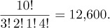
How many permutations of M are possible? If we regarded the elements of M as distinct, by subscripting them a₁, a₂, a₃, b₁, b₂, c₁, d₁, d₂, d₃, d₄, we would have 10! = 3,628,800 permutations; but many of those permutations would actually be the same when we removed the subscripts. In fact, each permutation of M would occur exactly 3! 2! 1! 4! = 288 times, since we can start with any permutation of M and put subscripts on the a’s in 3! ways, on the b’s (independently) in 2! ways, on the c in 1 way, and on the d’s in 4! ways. Therefore the true number of permutations of M is

In general, we can see by this same argument that the number of permutations of any multiset is the multinomial coefficient

Equation (3)

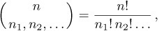
where n₁ is the number of elements of one kind, n₂ is the number of another kind, etc., and n = n₁ + n₂ + ... is the total number of elements.

The number of permutations of a set has been known for more than 1500 years. The Hebrew Book of Creation (c. A.D. 400), which was the earliest literary product of Jewish philosophical mysticism, gives the correct values of the first seven factorials, after which it says “Go on and compute what the mouth cannot express and the ear cannot hear.” [Sefer Yetzirah, end of Chapter 4. See Solomon Gandz, Studies in Hebrew Astronomy and Mathematics (New York: Ktav, 1970), 494–496; Aryeh Kaplan, Sefer Yetzirah (York Beach, Maine: Samuel Weiser, 1993).] This is one of the first two known enumerations of permutations in history. The other occurs in the Indian classic Anuyogadvārasūtra (c. 500), rule 97, which gives the formula

6 × 5 × 4 × 3 × 2 × 1 - 2

for the number of permutations of six elements that are neither in ascending nor descending order. [See G. Chakravarti, Bull. Calcutta Math. Soc. 24 (1932), 79–88. The Anuyogadvārasūtra is one of the books in the canon of Jainism, a religious sect that flourishes in India.]

The corresponding formula for permutations of multisets seems to have appeared first in the Līlāvatī of Bhāskara (c. 1150), sections 270–271. Bhāskara stated the rule rather tersely, and illustrated it only with two simple examples {2, 2, 1, 1} and {4, 8, 5, 5, 5}. Consequently the English translations of his work do not all state the rule correctly, although there is little doubt that Bhāskara knew what he was talking about. He went on to give the interesting formula

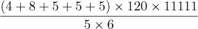
for the sum of the 20 numbers 48555 + 45855 + ....

The correct rule for counting permutations when elements are repeated was apparently unknown in Europe until Marin Mersenne stated it without proof as Proposition 10 in his elaborate treatise on melodic principles [Harmonie Universelle 2, also entitled Traitez de la Voix et des Chants (1636), 129–130]. Mersenne was interested in the number of tunes that could be made from a given collection of notes; he observed, for example, that a theme by Boesset,

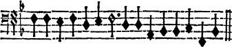
can be rearranged in exactly 15!/(4!3!3!2!) = 756,756,000 ways.

The general rule (3) also appeared in Jean Prestet’s Élémens des Mathématiques (Paris: 1675), 351–352, one of the very first expositions of combinatorial mathematics to be written in the Western world. Prestet stated the rule correctly for a general multiset, but illustrated it only in the simple case {a, a, b, b, c, c}. A few years later, John Wallis’s Discourse of Combinations (Oxford: 1685), Chapter 2 (published with his Treatise of Algebra) gave a clearer and somewhat more detailed discussion of the rule.

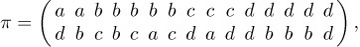
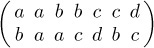
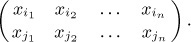
In 1965, Dominique Foata introduced an ingenious idea called the “intercalation product,” which makes it possible to extend many of the known results about ordinary permutations to the general case of multiset permutations. [See Publ. Inst. Statistique, Univ. Paris, 14 (1965), 81–241; also Lecture Notes in Math. 85 (Springer, 1969).] Assuming that the elements of a multiset have been linearly ordered in some way, we may consider a two-line notation such as

Equation (4)

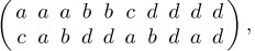
where the top line contains the elements of M sorted into nondecreasing order and the bottom line is the permutation itself. The intercalation product α β of two multiset permutations α and β is obtained by (a) expressing α and β in the two-line notation, (b) juxtaposing these two-line representations, and (c) sorting the columns into nondecreasing order of the top line. The sorting is supposed to be stable, in the sense that left-to-right order of elements in the bottom line is preserved when the corresponding top line elements are equal. For example, c a d a b b d d a d = c a b d d a b d a d, since

Equation (5)

It is easy to see that the intercalation product is associative:

Equation (6)

it also satisfies two cancellation laws:

Equation (7)

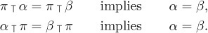
There is an identity element,

Equation (8)

where ∊ is the null permutation, the “arrangement” of the empty set. Although the commutative law is not valid in general (see exercise 2), we do have

Equation (9)

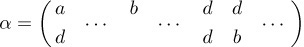
In an analogous fashion we can extend the concept of cycles in permutations to cases where elements are repeated; we let

Equation (10)

stand for the permutation obtained in two-line form by sorting the columns of

Equation (11)

by their top elements in a stable manner. For example, we have

so the permutation (4) is actually a cycle. We might render this cycle in words by saying something like “d goes to b goes to d goes to d goes . . . goes to d goes back.” Note that these general cycles do not share all of the properties of ordinary cycles; (x₁ x₂ . . . x_n) is not always the same as (x₂ . . . x_n x₁).

We observed in Section 1.3.3 that every permutation of a set has a unique representation (up to order) as a product of disjoint cycles, where the “product” of permutations is defined by a law of composition. It is easy to see that the product of disjoint cycles is exactly the same as their intercalation; this suggests that we might be able to generalize the previous results, obtaining a unique representation (in some sense) for any permutation of a multiset, as the intercalation of cycles. In fact there are at least two natural ways to do this, each of which has important applications.

Equation (5) shows one way to factor c a b d d a b d a d as the intercalation of shorter permutations; let us consider the general problem of finding all factorizations π = α β of a given permutation π. It will be helpful to consider a particular permutation, such as

Equation (12)

as we investigate the factorization problem.

If we can write this permutation π in the form α β, where α contains the letter a at least once, then the leftmost a in the top line of the two-line notation for α must appear over the letter d, so α must also contain at least one occurrence of the letter d. If we now look at the leftmost d in the top line of α, we see in the same way that it must appear over the letter d, so α must contain at least two d’s. Looking at the second d, we see that α also contains at least one b. We have deduced the partial result

Equation (13)

on the sole assumption that α is a left factor of π containing the letter a. Proceeding in the same manner, we find that the b in the top line of (13) must appear over the letter c, etc. Eventually this process will reach the letter a again, and we can identify this a with the first a if we choose to do so. The argument we have just made essentially proves that any left factor α of (12) that contains the letter a has the form (d d b c d b b c a) α′, for some permutation α′. (It is convenient to write the a last in the cycle, instead of first; this arrangement is permissible since there is only one a.) Similarly, if we had assumed that α contains the letter b, we would have deduced that α = (c d d b) α″ for some α″.

In general, this argument shows that, if we have any factorization α β = π, where α contains a given letter y, exactly one cycle of the form

Equation (14)

is a left factor of α. This cycle is easily determined when π and y are given; it is the shortest left factor of π that contains the letter y. One of the consequences of this observation is the following theorem:

Theorem A. Let the elements of the multiset M be linearly ordered by the relation “<”. Every permutation π of M has a unique representation as the intercalation

Equation (15)

where the following two conditions are satisfied:

Equation (16)

(In other words, the last element in each cycle is smaller than every other element, and the sequence of last elements is in nondecreasing order.)

Proof. If π = ∊, we obtain such a factorization by letting t = 0. Otherwise we let y₁ be the smallest element permuted; and we determine (x₁₁ . . . x_1n1y₁), the shortest left factor of π containing y₁, as in the example above. Now π = (x₁₁ . . . x_1n1 y₁) ρ for some permutation ρ; by induction on the length, we can write

where (16) is satisfied. This proves the existence of such a factorization.

Conversely, to prove that the representation (15) satisfying (16) is unique, clearly t = 0 if and only if π is the null permutation ∊. When t > 0, (16) implies that y₁ is the smallest element permuted, and that (x₁₁ . . . x_1n1 y₁) is the shortest left factor containing y₁. Therefore (x₁₁ . . . x_1n1 y₁) is uniquely determined; by the cancellation law (7) and induction, the representation is unique.

For example, the “canonical” factorization of (12), satisfying the given conditions, is

Equation (17)

if a < b < c < d.

It is important to note that we can actually drop the parentheses and the ’s in this representation, without ambiguity! Each cycle ends just after the first appearance of the smallest remaining element. So this construction associates the permutation

π′ = d d b c d b b c a b a c d b d

with the original permutation

π = d b c b c a c d a d d b b b d.

Whenever the two-line representation of π had a column of the form , where x < y, the associated permutation π′ has a corresponding pair of adjacent elements . . . y x . . . . Thus our example permutation π has three columns of the form , and π′ has three occurrences of the pair d b. In general this construction establishes the following remarkable theorem:

Theorem B. Let M be a multiset. There is a one-to-one correspondence between the permutations of M such that, if π corresponds to π′, the following conditions hold:

1. The leftmost element of π′ equals the leftmost element of π.
2. For all pairs of permuted elements (x, y) with x < y, the number of occurrences of the column in the two-line notation of π is equal to the number of times x is immediately preceded by y in π′.

When M is a set, this is essentially the same as the “unusual correspondence” we discussed near the end of Section 1.3.3, with unimportant changes. The more general result in Theorem B is quite useful for enumerating special kinds of permutations, since we can often solve a problem based on a two-line constraint more easily than the equivalent problem based on an adjacent-pair constraint.

P. A. MacMahon considered problems of this type in his extraordinary book Combinatory Analysis 1 (Cambridge Univ. Press, 1915), 168–186. He gave a constructive proof of Theorem B in the special case that M contains only two different kinds of elements, say a and b; his construction for this case is essentially the same as that given here, although he expressed it quite differently. For the case of three different elements a, b, c, MacMahon gave a complicated nonconstructive proof of Theorem B; the general case was first proved constructively by Foata [Comptes Rendus Acad. Sci. 258 (Paris, 1964), 1672–1675].

As a nontrivial example of Theorem B, let us find the number of strings of letters a, b, c containing exactly

Equation (18)

The theorem tells us that this is the same as the number of two-line arrays of the form

Equation (19)

The a’s can be placed in the second line in

then the b’s can be placed in the remaining positions in

The positions that are still vacant must be filled by c’s; hence the desired number is

Equation (20)

Let us return to the question of finding all factorizations of a given permutation. Is there such a thing as a “prime” permutation, one that has no intercalation factors except itself and ∊? The discussion preceding Theorem A leads us quickly to conclude that a permutation is prime if and only if it is a cycle with no repeated elements. For if it is such a cycle, our argument proves that there are no left factors except ∊ and the cycle itself. And if a permutation contains a repeated element y, it has a nontrivial cyclic left factor in which y appears only once.

A nonprime permutation can be factored into smaller and smaller pieces until it has been expressed as a product of primes. Furthermore we can show that the factorization is unique, if we neglect the order of factors that commute:

Theorem C. Every permutation of a multiset can be written as a product

Equation (21)

where each σ_j is a cycle having no repeated elements. This representation is unique, in the sense that any two such representations of the same permutation may be transformed into each other by successively interchanging pairs of adjacent disjoint cycles.

The term “disjoint cycles” means cycles having no elements in common. As an example of this theorem, we can verify that the permutation

has exactly five factorizations into primes, namely

Equation (22)

Proof. We must show that the stated uniqueness property holds. By induction on the length of the permutation, it suffices to prove that if ρ and σ are unequal cycles having no repeated elements, and if

• ρ α = σ β,

then ρ and σ are disjoint, and

• α = σ θ,      β = ρ θ,

for some permutation θ.

If y is any element of the cycle ρ, then any left factor of σ β containing the element y must have ρ as a left factor. So if ρ and σ have an element in common, σ is a multiple of ρ; hence σ = ρ (since they are primes), contradicting our assumption. Therefore the cycle containing y, having no elements in common with σ, must be a left factor of β. The proof is completed by using the cancellation law (7).

As an example of Theorem C, let us consider permutations of the multiset M = {A · a, B· b, C· c} consisting of A a’s, B b’s, and C c’s. Let N(A, B, C, m) be the number of permutations of M whose two-line representation contains no columns of the forms , and exactly m columns of the form . It follows that there are exactly A − m columns of the form , B − m of the form , C − B + m of the form , C − A + m of the form , and A + B − C − m of the form . Hence

Equation (23)

Theorem C tells us that we can count these permutations in another way: Since columns of the form are excluded, the only possible prime factors of the permutation are

Equation (24)

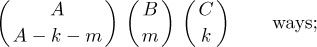
Each pair of these cycles has at least one letter in common, so the factorization into primes is completely unique. If the cycle (a b c) occurs k times in the factorization, our previous assumptions imply that (a b) occurs m − k times, (b c) occurs C − A + m − k times, (a c) occurs C − B + m − k times, and (a c b) occurs A + B − C − 2m + k times. Hence N(A, B, C, m) is the number of permutations of these cycles (a multinomial coefficient), summed over k:

N(A, B, C, m)

Equation (25)

Comparing this with (23), we find that the following identity must be valid:

Equation (26)

This turns out to be the identity we met in exercise 1.2.6–31, namely

Equation (27)

with M = A+B–C–m, N = C–B+m, R = B, S = C, and j = C–B+m–k.

Similarly we can count the number of permutations of {A·a, B·b, C·c, D·d} such that the number of columns of various types is specified as follows:

Equation (28)

(Here A + C = B + D.) The possible cycles occurring in a prime factorization of such permutations are then

Equation (29)

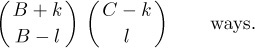
for some s (see exercise 12). In this case the cycles (a b) and (c d) commute with each other, and so do (b c) and (d a), so we must count the number of distinct prime factorizations. It turns out (see exercise 10) that there is always a unique factorization such that no (c d) is immediately followed by (a b), and no (d a) is immediately followed by (b c). Hence by the result of exercise 13, we have

Taking out the factor from both sides and simplifying the factorials slightly leaves us with the complicated-looking five-parameter identity

Equation (30)

The sum on s can be performed using (27), and the resulting sum on t is easily evaluated; so, after all this work, we were not fortunate enough to discover any identities that we didn’t already know how to derive. But at least we have learned how to count certain kinds of permutations, in two different ways, and these counting techniques are good training for the problems that lie ahead.

Exercises

• 1. [M05] True or false: Let M₁ and M₂ be multisets. If α is a permutation of M₁ and β is a permutation of M₂, then α β is a permutation of M₁ ∪ M₂.
• 2. [10] The intercalation of c a d a b and b d d a d is computed in (5); find the intercalation b d d a d c a d a b that is obtained when the factors are interchanged.
• 3. [M13] Is the converse of (9) valid? In other words, if α and β commute under intercalation, must they have no letters in common?
• 4. [M11] The canonical factorization of (12), in the sense of Theorem A, is given in (17) when a < b < c < d. Find the corresponding canonical factorization when d < c < b < a.
• 5. [M23] Condition (b) of Theorem B requires x < y; what would happen if we weakened the relation to x ≤ y?
• 6. [M15] How many strings are there that contain exactly m a’s, n b’s, and no other letters, with exactly k of the a’s preceded immediately by a b?
• 7. [M21] How many strings on the letters a, b, c satisfying conditions (18) begin with the letter a? with the letter b? with c?
• ▸ 8. [20] Find all factorizations of (12) into two factors α β.
• 9. [33] Write computer programs that perform the factorizations of a given multiset permutation into the forms mentioned in Theorems A and C.
• ▸ 10. [M30] True or false: Although the factorization into primes isn’t quite unique, according to Theorem C, we can ensure uniqueness in the following way: “There is a linear ordering of the set of primes such that every permutation of a multiset has a unique factorization σ₁ σ₂ · · · σ_n into primes subject to the condition that σ_i σ_i+1 whenever σ_i commutes with σ_i+1, for 1 ≤ i < n.”
• ▸ 11. [M26] Let σ₁, σ₂, . . ., σ_t be cycles without repeated elements. Define a partial ordering on the t objects {x₁, . . ., x_t} by saying that x_i x_j if i < j and σ_i has at least one letter in common with σ_j. Prove the following connection between Theorem C and the notion of “topological sorting” (Section 2.2.3): The number of distinct prime factorizations of σ₁σ₂· · ·σ_t is the number of ways to sort the given partial ordering topologically. (For example, corresponding to (22) we find that there are five ways to sort the ordering x₁ x₂, x₃ x₄, x₁ x₄ topologically.) Conversely, given any partial ordering on t elements, there is a set of cycles {σ₁, σ₂, . . ., σ_t} that defines it in the stated way.
• 12. [M16] Show that (29) is a consequence of the assumptions of (28).

• 13. [M21] Prove that the number of permutations of the multiset

  {A· a, B· b, C· c, D· d, E· e, F· f}

  containing no occurrences of the adjacent pairs of letters ca and db is

  

  Click to view larger image

• 14. [M30] One way to define the inverse π⁻ of a general permutation π, suggested by other definitions in this section, is to interchange the lines of the two-line representation of π and then to do a stable sort of the columns in order to bring the top row into nondecreasing order. For example, if a < b < c < d, this definition implies that the inverse of c a b d d a b d a d is a c d a d a b b d d.

  Explore properties of this inversion operation; for example, does it have any simple relation with intercalation products? Can we count the number of permutations such that π = π⁻?

• ▸15. [M25] Prove that the permutation a₁ . . . a_n of the multiset

  {n₁ · x₁, n₂ · x₂, . . ., n_m · x_m},

  where x₁ < x₂ < · · · < x_m and n₁ + n₂ + · · · + n_m = n, is a cycle if and only if the directed graph with vertices {x₁, x₂, . . ., x_m} and arcs from x_j to a_n1+···+nj contains precisely one oriented cycle. In the latter case, the number of ways to represent the permutation in cycle form is the length of the oriented cycle. For example, the directed graph corresponding to

  

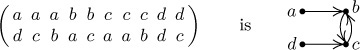
  and the two ways to represent the permutation as a cycle are (b a d d c a c a b c) and (c a d d c a c b a b).

• 16. [M35] We found the generating function for inversions of permutations in the previous section, Eq. 5.1.1–(8), in the special case that a set was being permuted. Show that, in general, if a multiset is permuted, the generating function for inversions of {n₁ · x₁, n₂ · x₂, . . . } is the “z-multinomial coefficient”

  

  Click to view larger image

  [Compare with (3) and with the definition of z-nomial coefficients in Eq. 1.2.6–(40).]

• 17. [M24] Find the average and standard deviation of the number of inversions in a random permutation of a given multiset, using the generating function found in exercise 16.
• 18. [M30] (P. A. MacMahon.) The index of a permutation a₁ a₂ . . . a_n was defined in the previous section; and we proved that the number of permutations of a given set that have a given index k is the same as the number of permutations that have k inversions. Does the same result hold for permutations of a given multiset?

• 19. [HM28] Define the Möbius function µ(π) of a permutation π to be 0 if π contains repeated elements, otherwise (−1)^k if π is the product of k primes. (Compare with the definition of the ordinary Möbius function, exercise 4.5.2–10.)

  1. Prove that if π ≠ , we have

     ∑µ(λ) = 0,

     summed over all permutations λ that are left factors of π (namely all λ such that π = λ ρ for some ρ).

  2. b) Given that x₁ < x₂ < · · · < x_m and π = x_i1 x_i2 . . . x_in, where 1 ≤ i_k ≤ m for 1 ≤ k ≤ n, prove that

     

     Click to view larger image

• ▸ 20. [HM33] (D. Foata.) Let (a_ij) be any matrix of real numbers. In the notation of exercise 19(b), define ν(π) = a_i1j1 . . . a_injn, where the two-line notation for π is

  

  This function is useful in the computation of generating functions for permutations of a multiset, because ∑ν(π), summed over all permutations π of the multiset

  {n₁ · x₁, . . ., n_m · x_m},

  will be the generating function for the number of permutations satisfying certain restrictions. For example, if we take a_ij = z for i = j, and a_ij = 1 for i ≠ j, then ∑ν(π) is the generating function for the number of “fixed points” (columns in which the top and bottom entries are equal). In order to study ∑ν(π) for all multisets simultaneously, we consider the function

  G = ∑πν(π)

  summed over all π in the set {x₁, . . ., x_m}* of all permutations of multisets involving the elements x₁, . . ., x_m, and we look at the coefficient of in G.

  In this formula for G we are treating π as the product of the x’s. For example, when m = 2 we have

  

  Click to view larger image

  Thus the coefficient of in G is ∑ν(π) summed over all permutations π of {n₁ · x₁, . . ., n_m · x_m}. It is not hard to see that this coefficient is also the coefficient of in the expression

  (a₁₁x₁ + · · · + a_1mx_m)ⁿ₁ (a₂₁x₁ + · · · + a_2mx_m)^n₂ . . . (a_m1x₁ + · · · + a_mmx_m)ⁿ_m .

  The purpose of this exercise is to prove what P. A. MacMahon called a “Master Theorem” in his Combinatory Analysis 1 (1915), Section 3, namely the formula

  

  Click to view larger image

  For example, if a_ij = 1 for all i and j, this formula gives

  G = 1/(1 − (x₁ + x₂ + · · · + x_m)),

  and the coefficient of turns out to be (n₁ + · · · + n_m)!/n₁! . . . n_m!, as it should. To prove the Master Theorem, show that

  1. ν(π ρ) = ν(π)ν(ρ);
  2. D = ∑πµ(π)ν(π), in the notation of exercise 19, summed over all permutations π in {x₁, . . ., x_m}*;
  3. c) therefore D · G = 1.
• 21. [M21] Given n₁, . . ., n_m, and d ≥ 0, how many permutations a₁ a₂ . . . a_n of the multiset {n₁ · 1, . . ., n_m · m} satisfy a_j+1 ≥ a_j − d for 1 ≤ j < n = n₁ + · · · + n_m?

• 22. [M30] Let P() denote the set of all possible permutations of the multiset {n₁ ·x₁, . . ., n_m ·x_m}, and let P₀() be the subset of P() in which the first n₀ elements are ≠ x₀.

  1. Given a number t with 1 ≤ t < m, find a one-to-one correspondence between P (1^n₁ . . . m^n_m) and the set of all ordered pairs of permutations that belong respectively to P₀(0^p1^n₁ . . . t^n_t) and P₀(0^p(t+1)^n_t+1 . . . m^n_m), for some p ≥ 0. [Hint: For each π = a₁ . . . a_n ∈ P (1^n₁ . . . m^n_m), let l(π) be the permutation obtained by replacing t + 1, . . ., m by 0 and erasing all 0s in the last n_t+1 + · · · + n_m positions; similarly, let r(π) be the permutation obtained by replacing 1, . . ., t by 0 and erasing all 0s in the first n₁ + · · · + n_t positions.]

  2. Prove that the number of permutations of P₀(0ⁿ₀ 1ⁿ₁ . . . m^n_m) whose two-line form has p_j columns and q_j columns is

     

     Click to view larger image

  3. Let w₁, . . ., w_m, z₁, . . ., z_m be complex numbers on the unit circle. Define the weight w(π) of a permutation π ∈ P (1^n₁ . . . m^n_m) as the product of the weights of its columns in two-line form, where the weight of is w_j/w_k if j and k are both ≤ t or both > t, otherwise it is z_j/z_k. Prove that the sum of w(π) over all π ∈ P (1ⁿ₁ . . . m^n_m) is

     

     Click to view larger image

     where n_≤t is n₁ + · · · + n_t, n_>t is n_t+1 + · · · + n_m, and the inner sum is over all (p₁, . . ., p_m) such that p_≤t = p_>t = p.

• 23. [M23] A strand of DNA can be thought of as a word on a four-letter alphabet. Suppose we copy a strand of DNA and break it completely into one-letter bases, then recombine those bases at random. If the resulting strand is placed next to the original, prove that the number of places in which they differ is more likely to be even than odd. [Hint: Apply the previous exercise.]

• 24. [27] Consider any relation R that might hold between two unordered pairs of letters; if {w, x}R{y, z} we say {w, x} preserves {y, z}, otherwise {w, x} moves {y, z}.

  The operation of transposing with respect to R replaces by or , according as the pair {w, x} preserves or moves the pair {y, z}, assuming that w ≠ x and y ≠ z; if w = x or y = z the transposition always produces .

  The operation of sorting a two-line array () with respect to R repeatedly finds the largest x_j such that x_j > x_j+1 and transposes columns j and j + 1, until eventually x₁ ≤ · · · ≤ x_n. (We do not require y₁ . . . y_n to be a permutation of x₁ . . . x_n.)

  1. Given (), prove that for every x ∈ {x₁, . . ., x_n} there is a unique y ∈ {y₁, . . ., y_n} such that sort () = sort () for some .

  2. Let denote the result of sorting () with respect to R. For example, if R is always true, sorts {w₁, . . ., w_k, x₁, . . ., x_l}, but it simply juxtaposes y₁ . . . y_k with z₁ . . . z_l; if R is always false, is the intercalation product . Generalize Theorem A by proving that every permutation π of a multiset M has a unique representation of the form

     

     Click to view larger image

     satisfying (16), if we redefine cycle notation by letting the two-line array (11) correspond to the cycle (x₂ . . . x_n x₁) instead of to (x₁ x₂ . . . x_n). For example, suppose {w, x}R{y, z} means that w, x, y, and z are distinct; then it turns out that the factorization of (12) analogous to (17) is

     

     Click to view larger image

     (The operation does not always obey the associative law; parentheses in the generalized factorization should be nested from right to left.)