This chapter is from the book
This chapter is from the book
This chapter is from the book
15.4. A Ray-Casting Renderer
We begin the ray-casting renderer by expanding and implementing our initial pseudocode from Listing 15.2. It is repeated in Listing 15.11 with more detail.
Listing 15.11: Detailed pseudocode for a ray-casting renderer.
 1  for each pixel row y:
 2     for each pixel column x:
 3        let R = ray through screen space position (x + 0.5, y + 0.5)
 4        closest = ∞
 5        for each triangle T:
 6           d = intersect(T, R)
 7           if (d < closest)
 8               closest = d
 9               sum = 0
10               let P be the intersection point
11               for each direction ωi:
12                  sum += light scattered at P from ωi to ωo
13
14               image[x, y] = sum
The three loops iterate over every ray and triangle combination. The body of the for-each-triangle loop verifies that the new intersection is closer than previous observed ones, and then shades the intersection. We will abstract the operation of ray intersection and sampling into a helper function called sampleRayTriangle. Listing 15.12 gives the interface for this helper function.
Listing 15.12: Interface for a function that performs ray-triangle intersection and shading.
1boolsampleRayTriangle(constScene& scene,intx,inty, 2constRay& R,constTriangle& T, 3 Radiance3& radiance,float& distance);
The specification for sampleRayTriangle is as follows. It tests a particular ray against a triangle. If the intersection exists and is closer than all previously observed intersections for this ray, it computes the radiance scattered toward the viewer and returns true. The innermost loop therefore sets the value of pixel (x, y) to the radiance L_o passing through its center from the closest triangle. Radiance from farther triangles is not interesting because it will (conceptually) be blocked by the back of the closest triangle and never reach the image. The implementation of sampleRayTriangle appears in Listing 15.15.
To render the entire image, we must invoke sampleRayTriangle once for each pixel center and for each triangle. Listing 15.13 defines rayTrace, which performs this iteration. It takes as arguments a box within which to cast rays (see Section 15.4.4). We use L_o to denote the radiance from the triangle; the subscript “o” is for “outgoing”.
Listing 15.13: Code to trace one ray for every pixel between (x0, y0) and (x1-1, y1-1), inclusive.
1/** Trace eye rays with origins in the box from [x0, y0] to (x1, y1).*/2voidrayTrace(Image& image,constScene& scene, 3constCamera& camera,intx0,intx1,inty0,inty1) { 4 5// For each pixel6 for (inty = y0; y < y1; ++y) { 7 for (intx = y0; x < x1; ++x) { 8 9// Ray through the pixel10constRay& R = computeEyeRay(x + 0.5f, y + 0.5f, image.width(), 11 image.height(), camera); 12 13// Distance to closest known intersection14floatdistance = INFINITY; 15 Radiance3 L_o; 16 17// For each triangle18for(unsigned intt = 0; t < scene.triangleArray.size(); ++t){ 19constTriangle& T = scene.triangleArray[t]; 20 21if(sampleRayTriangle(scene, x, y, R, T, L_o, distance)) { 22 image.set(x, y, L_o); 23 } 24 } 25 } 26 } 27 }
To invoke rayTrace on the entire image, we will use the call:
rayTrace(image, scene, camera, 0, image.width(), 0, image.height());
15.4.1. Generating an Eye Ray
Assume the camera’s center of projection is at the origin, (0, 0, 0), and that, in the camera’s frame of reference, the y-axis points upward, the x-axis points to the right, and the z-axis points out of the screen. Thus, the camera is facing along its own –z-axis, in a right-handed coordinate system. We can transform any scene to this coordinate system using the transformations from Chapter 11.
We require a utility function, computeEyeRay, to find the ray through the center of a pixel, which in screen space is given by (x + 0.5, y + 0.5) for integers x and y. Listing 15.14 gives an implementation. The key geometry is depicted in Figure 15.3. The figure is a top view of the scene in which x increases to the right and z increases downward. The near plane appears as a horizontal line, and the start point is on that plane, along the line from the camera at the origin to the center of a specific pixel.
To implement this function we needed to parameterize the camera by either the image plane depth or the desired field of view. Field of view is a more intuitive way to specify a camera, so we previously chose that parameterization when building the scene representation.
Listing 15.14: Computing the ray through the center of pixel (x, y) on a width × height image.
1 Ray computeEyeRay(floatx,floaty,intwidth,intheight,constCamera& camera) { 2const floataspect = float(height) / width; 3 4// Compute the side of a square at z = -1 based on our5// horizontal left-edge-to-right-edge field of view6const floats = -2.0f * tan(camera.fieldOfViewX * 0.5f); 7 8constVector3& start = 9 Vector3( (x / width - 0.5f) * s, 10 -(y / height - 0.5f) * s * aspect, 1.0f) * camera.zNear; 11 12returnRay(start, start.direction()); 13 }
We choose to place the ray origin on the near (sometimes called hither) clipping plane, at z = camera.zNear. We could start rays at the origin instead of the near plane, but starting at the near plane will make it easier for results to line up precisely with our rasterizer later.
The ray direction is the direction from the center of projection (which is at the origin, (0, 0, 0)) to the ray start point, so we simply normalize start point.
Note that the y-coordinate of the start is negated. This is because y is in 2D screen space, with a “y = down” convention, and the ray is in a 3D coordinate system with a “y = up” convention.
To specify the vertical field of view instead of the horizontal one, replace fieldOfViewX with fieldOfViewY and insert the line s /= aspect.
15.4.1.1. Camera Design Notes
The C++ language offers both functions and methods as procedural abstractions. We have presented computeEyeRay as a function that takes a Camera parameter to distinguish the “support code” Camera class from the ray-tracer-specific code that you are adding. As you move forward through the book, consider refactoring the support code to integrate auxiliary functions like this directly into the appropriate classes. (If you are using an existing 3D library as support code, it is likely that the provided camera class already contains such a method. In that case, it is worth implementing the method once as a function here so that you have the experience of walking through and debugging the routine. You can later discard your version in favor of a canonical one once you’ve reaped the educational value.)
A software engineering tip: Although we have chosen to forgo small optimizations, it is still important to be careful to use references (e.g., Image&) to avoid excess copying of arguments and intermediate results. There are two related reasons for this, and neither is about the performance of this program.
The first reason is that we want to be in the habit of avoiding excessive copying. A Vector3 occupies 12 bytes of memory, but a full-screen Image is a few megabytes. If we’re conscientious about never copying data unless we want copy semantics, then we won’t later accidentally copy an Image or other large structure. Memory allocation and copy operations can be surprisingly slow and will bloat the memory footprint of our program. The time cost of copying data isn’t just a constant overhead factor on performance. Copying the image once per pixel, in the inner loop, would change the ray caster’s asymptotic run time from Ο(n) in the number of pixels to Ο(n2).
The second reason is that experienced programmers rely on a set of idioms that are chosen to avoid bugs. Any deviation from those attracts attention, because it is a potential bug. One such convention in C++ is to pass each value as a const reference unless otherwise required, for the long-term performance reasons just described. So code that doesn’t do so takes longer for an experienced programmer to review because of the need to check that there isn’t an error or performance implication whenever an idiom is not followed. If you are an experienced C++ programmer, then such idioms help you to read the code. If you are not, then either ignore all the ampersands and treat this as pseudocode, or use it as an opportunity to become a better C++ programmer.
15.4.1.2. Testing the Eye-Ray Computation
We need to test computeEyeRay before continuing. One way to do this is to write a unit test that computes the eye rays for specific pixels and then compares them to manually computed results. That is always a good testing strategy. In addition to that, we can visualize the eye rays. Visualization is a good way to quickly see the result of many computations. It allows us to more intuitively check results, and to identify patterns of errors if they do not match what we expected.
In this section, we’ll visualize the directions of the rays. The same process can be applied to the origins. The directions are the more common location for an error and conveniently have a bounded range, which make them both more important and easier to visualize.
A natural scheme for visualizing a direction is to interpret the (x, y, z) fields as (r, g, b) color triplets. The conversion of ray direction to pixel color is of course a gross violation of units, but it is a really useful debugging technique and we aren’t expecting anything principled here anyway.
Because each ordinate is on the interval [–1, 1], we rescale them to the range [0, 1] by r = (x + 1)/2. Our image display routines also apply an exposure function, so we need to scale the resultant intensity down by a constant on the order of the inverse of the exposure value. Temporarily inserting the following line:
image.set(x, y, Color3(R.direction() + Vector3(1, 1, 1)) / 5);
into rayTrace in place of the sampleRayTriangle call should yield an image like that shown in Figure 15.4. (The factor of 1/5 scales the debugging values to a reasonable range for our output, which was originally calibrated for radiance; we found a usable constant for this particular example by trial and error.) We expect the x-coordinate of the ray, which here is visualized as the color red, to increase from a minimum on the left to a maximum on the right. Likewise, the (3D) y-coordinate, which is visualized as green, should increase from a minimum at the bottom of the image to a maximum at the top. If your result varies from this, examine the pattern you observe and consider what kind of error could produce it. We will revisit visualization as a debugging technique later in this chapter, when testing the more complex intersection routine.
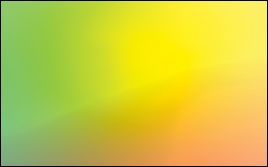
Figure 15.4: Visualization of eyeray directions.
15.4.2. Sampling Framework: Intersect and Shade
Listing 15.15 shows the code for sampling a triangle with a ray. This code doesn’t perform any of the heavy lifting itself. It just computes the values needed for intersect and shade.
Listing 15.15: Sampling the intersection and shading of one triangle with one ray.
1boolsampleRayTriangle(constScene& scene,intx,inty,constRay& R,constTriangle& T, Radiance3& radiance, float& distance) { 2 3floatweight[3]; 4const floatd = intersect(R, T, weight); 5 6if(d >= distance) { 7return false; 8 } 9 10// This intersection is closer than the previous one11 distance = d; 12 13// Intersection point14constPoint3& P = R.origin() + R.direction() * d; 15 16// Find the interpolated vertex normal at the intersection17constVector3& n = (T.normal(0) * weight[0] + 18 T.normal(1) * weight[1] + 19 T.normal(2) * weight[2]).direction(); 20 21constVector3& w_o = -R.direction(); 22 23 shade(scene, T, P, n, w_o, radiance); 24 25// Debugging intersect: set to white on any intersection26//radiance = Radiance3(1, 1, 1);27 28// Debugging barycentric29//radiance = Radiance3(weight[0], weight[1], weight[2]) / 15;30 31return true; 32 }
The sampleRayTriangle routine returns false if there was no intersection closer than distance; otherwise, it updates distance and radiance and returns true.
When invoking this routine, the caller passes the distance to the closest currently known intersection, which is initially INFINITY (let INFINITY = std::numeric_limits<T>::infinity() in C++, or simply 1.0/0.0). We will design the intersect routine to return INFINITY when no intersection exists between R and T so that a missed intersection will never cause sampleRayTriangle to return true.
Placing the (d >= distance) test before the shading code is an optimization. We would still obtain correct results if we always computed the shading before testing whether the new intersection is in fact the closest. This is an important optimization because the shade routine may be arbitrarily expensive. In fact, in a full-featured ray tracer, almost all computation time is spent inside shade, which recursively samples additional rays. We won’t discuss further shading optimizations in this chapter, but you should be aware of the importance of an early termination when another surface is known to be closer.
Note that the order of the triangles in the calling routine (rayTrace) affects the performance of the routine. If the triangles are in back-to-front order, then we will shade each one, only to reject all but the closest. This is the worst case. If the triangles are in front-to-back order, then we will shade the first and reject the rest without further shading effort. We could ensure the best performance always by separating sampleRayTriangle into two auxiliary routines: one to find the closest intersection and one to shade that intersection. This is a common practice in ray tracers. Keep this in mind, but do not make the change yet. Once we have written the rasterizer renderer, we will consider the space and time implications of such optimizations under both ray casting and rasterization, which gives insights into many variations on each algorithm.
We’ll implement and test intersect first. To do so, comment out the call to shade on line 23 and uncomment either of the debugging lines below it.
15.4.3. Ray-Triangle Intersection
We’ll find the intersection of the eye ray and a triangle in two steps, following the method described in Section 7.9 and implemented in Listing 15.16. This method first intersects the line containing the ray with the plane containing the triangle. It then solves for the barycentric weights to determine if the intersection is within the triangle. We need to ignore intersections with the back of the single-sided triangle and intersections that occur along the part of the line that is not on the ray.
The same weights that we use to determine if the intersection is within the triangle are later useful for interpolating per-vertex properties, such as shading normals. We structure our implementation to return the weights to the caller. The caller could use either those or the distance traveled along the ray to find the intersection point. We return the distance traveled because we know that we will later need that anyway to identify the closest intersection to the viewer in a scene with many triangles. We return the barycentric weights for use in interpolation.
Figure 15.5 shows the geometry of the situation. Let R be the ray and T be the triangle. Let  be the edge vector from V0 to V1 and
  be the edge vector from V0 to V2. Vector
  is orthogonal to both the ray and . Note that if is also orthogonal to , then the ray is parallel to the triangle and there is no intersection. If is in the negative hemisphere of (i.e., “points away”), then the ray travels away from the triangle.
)
Figure 15.5: Variables for computing the intersection of a ray and a triangle (see Listing 15.16).
Vector  is the displacement of the ray origin from V0, and vector
  is the cross product of and . These vectors are used to construct the barycentric weights, as shown in Listing 15.16.
Variable a is the rate at which the ray is approaching the triangle, multiplied by twice the area of the triangle. This is not obvious from the way it is computed here, but it can be seen by applying a triple-product identity relation:
)
)
since the direction of  2 × 1 is opposite the triangle’s geometric normal n. The particular form of this expression chosen in the implementation is convenient because the q vector is needed again later in the code for computing the barycentric weights.
There are several cases where we need to compare a value against zero. The two epsilon constants guard these comparisons against errors arising from limited numerical precision.
The comparison a <= epsilon detects two cases. If a is zero, then the ray is parallel to the triangle and never intersects it. In this case, the code divided by zero many times, so other variables may be infinity or not-a-number. That’s irrelevant, since the first test expression will still make the entire test expression true. If a is negative, then the ray is traveling away from the triangle and will never intersect it. Recall that a is the rate at which the ray approaches the triangle, multiplied by the area of the triangle. If epsilon is too large, then intersections with triangles will be missed at glancing angles, and this missed intersection behavior will be more likely to occur at triangles with large areas than at those with small areas. Note that if we changed the test to fabs(a)<= epsilon, then triangles would have two sides. This is not necessary for correct models of real, opaque objects; however, for rendering mathematical models or models with errors in them it can be convenient. Later we will depend on optimizations that allow us to quickly cull the (approximately half) of the scene representing back faces, so we choose to render single-sided triangles here for consistency.
Listing 15.16: Ray-triangle intersection (derived from [MT97])
1floatintersect(constRay& R,constTriangle& T,floatweight[3]) { 2constVector3& e1 = T.vertex(1) - T.vertex(0); 3constVector3& e2 = T.vertex(2) - T.vertex(0); 4constVector3& q = R.direction().cross(e2); 5 6const floata = e1.dot(q); 7 8constVector3& s = R.origin() - T.vertex(0); 9constVector3& r = s.cross(e1); 10 11// Barycentric vertex weights12 weight[1] = s.dot(q) / a; 13 weight[2] = R.direction().dot(r) / a; 14 weight[0] = 1.0f - (weight[1] + weight[2]); 15 16const floatdist = e2.dot(r) / a; 17 18 staticconst floatepsilon = 1e-7f; 19 staticconst floatepsilon2 = 1e-10; 20 21 if ((a <= epsilon) || (weight[0] < -epsilon2) || 22 (weight[1] < -epsilon2) || (weight[2] < -epsilon2) || 23 (dist <= 0.0f)) { 24// The ray is nearly parallel to the triangle, or the25// intersection lies outside the triangle or behind26// the ray origin: "infinite" distance until intersection.27returnINFINITY; 28 }else{ 29returndist; 30 } 31 }
The epsilon2 constant allows a ray to intersect a triangle slightly outside the bounds of the triangle. This ensures that triangles that share an edge completely cover pixels along that edge despite numerical precision limits. If epsilon2 is too small, then single-pixel holes will very occasionally appear on that edge. If it is too large, then all triangles will visibly appear to be too large.
Depending on your processor architecture, it may be faster to perform an early test and potential return rather than allowing not-a-number and infinity propagation in the ill-conditioned case where a ≈ 0. Many values can also be precomputed, for example, the edge lengths of the triangle, or at least be reused within a single intersection, for example, 1.0f / a. There’s a cottage industry of optimizing this intersection code for various architectures, compilers, and scene types (e.g., [MT97] for scalar processors versus [WBB08] for vector processors). Let’s forgo those low-level optimizations and stick to high-level algorithmic decisions. In practice, most ray casters spend very little time in the ray intersection code anyway. The fastest way to determine if a ray intersects a triangle is to never ask that question in the first place. That is, in Chapter 37, we will introduce data structures that quickly and conservatively eliminate whole sets of triangles that the ray could not possibly intersect, without ever performing the ray-triangle intersection. So optimizing this routine now would only complicate it without affecting our long-term performance profile.
Our renderer only processes triangles. We could easily extend it to render scenes containing any kind of primitive for which we can provide a ray intersection solution. Surfaces defined by low-order equations, like the plane, rectangle, sphere, and cylinder, have explicit solutions. For others, such as bicubic patches, we can use root-finding methods.
15.4.4. Debugging
We now verify that the intersection code code is correct. (The code we’ve given you is correct, but if you invoked it with the wrong parameters, or introduced an error when porting to a different language or support code base, then you need to learn how to find that error.) This is a good opportunity for learning some additional graphics debugging tricks, all of which demonstrate the Visual Debugging principle.
It would be impractical to manually examine every intersection result in a debugger or printout. That is because the rayTrace function invokes intersect thousands of times. So instead of examining individual results, we visualize the barycentric coordinates by setting the radiance at a pixel to be proportional to the barycentric coordinates following the Visual Debugging principle. Figure 15.6 shows the correct resultant image. If your program produces a comparable result, then your program is probably nearly correct.
)
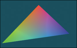
Figure 15.6: The single triangle scene visualized with color equal to barycentric weight for debugging the intersection code.
What should you do if your result looks different? You can’t examine every result, and if you place a breakpoint in intersect, then you will have to step through hundreds of ray casts that miss the triangle before coming to the interesting intersection tests.
This is why we structured rayTrace to trace within a caller-specified rectangle, rather than the whole image. We can invoke the ray tracer on a single pixel from main(), or better yet, create a debugging interface where clicking on a pixel with the mouse invokes the single-pixel trace on the selected pixel. By setting breakpoints or printing intermediate results under this setup, we can investigate why an artifact appears at a specific pixel. For one pixel, the math is simple enough that we can also compute the desired results by hand and compare them to those produced by the program.
In general, even simple graphics programs tend to have large amounts of data. This may be many triangles, many pixels, or many frames of animation. The processing for these may also be running on many threads, or on a GPU. Traditional debugging methods can be hard to apply in the face of such numerous data and massive parallelism. Furthermore, the graphics development environment may preclude traditional techniques such as printing output or setting breakpoints. For example, under a hardware rendering API, your program is executing on an embedded processor that frequently has no access to the console and is inaccessible to your debugger.
Fortunately, three strategies tend to work well for graphics debugging.
- Use assertions liberally. These cost you nothing in the optimized version of the program, pass silently in the debug version when the program operates correctly, and break the program at the test location when an assertion is violated. Thus, they help to identify failure cases without requiring that you manually step through the correct cases.
- Immediately reduce to the minimal test case. This is often a single-triangle scene with a single light and a single pixel. The trick here is to find the combination of light, triangle, and pixel that produces incorrect results. Assertions and the GUI click-to-debug scheme work well for that.
- Visualize intermediate results. We have just rendered an image of the barycentric coordinates of eye-ray intersections with a triangle for a 400,000-pixel image. Were we to print out these values or step through them in the debugger, we would have little chance of recognizing an incorrect value in that mass of data. If we see, for example, a black pixel, or a white pixel, or notice that the red and green channels are swapped, then we may be able to deduce the nature of the error that caused this, or at least know which inputs cause the routine to fail.
15.4.5. Shading
We are now ready to implement shade. This routine computes the incident radiance at the intersection point P and how much radiance scatters back along the eye ray to the viewer.
Let’s consider only light transport paths directly from the source to the surface to the camera. Under this restriction, there is no light arriving at the surface from any directions except those to the lights. So we only need to consider a finite number of ωi values. Let’s also assume for the moment that there is always a line of sight to the light. This means that there will (perhaps incorrectly) be no shadows in the rendered image.
Listing 15.17 iterates over the light sources in the scene (note that we have only one in our test scene). For each light, the loop body computes the distance and direction to that light from the point being shaded. Assume that lights emit uniformly in all directions and are at finite locations in the scene. Under these assumptions, the incident radiance L_i at point P is proportional to the total power of the source divided by the square of the distance between the source and P. This is because at a given distance, the light’s power is distributed equally over a sphere of that radius. Because we are ignoring shadowing, let the visible function always return true for now. In the future it will return false if there is no line of sight from the source to P, in which case the light should contribute no incident radiance.
The outgoing radiance to the camera, L_o, is the sum of the fraction of incident radiance that scatters in that direction. We abstract the scattering function into a BSDF. We implement this function as a class so that it can maintain state across multiple invocations and support an inheritance hierarchy. Later in this book, we will also find that it is desirable to perform other operations beyond invoking this function; for example, we might want to sample with respect to the probability distribution it defines. Using a class representation will allow us to later introduce additional methods for these operations.
The evaluateFiniteScatteringDensity method of that class evaluates the scattering function for the given incoming and outgoing angles. We always then take the product of this and the incoming radiance, modulated by the cosine of the angle between w_i and n to account for the projected area over which incident radiance is distributed (by the Tilting principle).
Listing 15.17: The single-bounce shading code.
1voidshade(constScene& scene,constTriangle& T,constPoint3& P,constVector3& n,constVector3& w_o,Radiance3& L_o) { 2 3 L_o =Color3(0.0f, 0.0f, 0.0f); 4 5// For each direction (to a light source)6for(unsigned inti = 0; i < scene.lightArray.size(); ++i) { 7constLight& light = scene.lightArray[i]; 8 9constVector3& offset = light.position - P; 10const floatdistanceToLight = offset.length(); 11constVector3& w_i = offset / distanceToLight; 12 13 if (visible(P, w_i, distanceToLight, scene)) { 14constRadiance3& L_i = light.power / (4 * PI * square(distanceToLight)); 15 16// Scatter the light17 L_o += 18 L_i * 19 T.bsdf(n).evaluateFiniteScatteringDensity(w_i, w_o) * 20 max(0.0, dot(w_i, n)); 21 } 22 } 23 }
15.4.6. Lambertian Scattering
The simplest implementation of the BSDF assumes a surface appears to be the same brightness independent of the viewer’s orientation. That is, evaluateFiniteScatteringDensity returns a constant. This is called Lambertian reflectance, and it is a good model for matte surfaces such as paper and flat wall paint. It is also trivial to implement. Listing 15.18 gives the implementation (see Section 14.9.1 for a little more detail and Chapter 29 for a lot more). It has a single member, lambertian, that is the “color” of the surface. For energy conservation, this value should have all fields on the range [0, 1].
Listing 15.18: Lambertian BSDF implementation, following Listing 14.6.
1classBSDF{ 2public: 3Color3k_L; 4 5/** Returns f = L_o / (L_i * w_i.dot(n)) assuming6incident and outgoing directions are both in the7positive hemisphere above the normal */8Color3evaluateFiniteScatteringDensity 9 (constVector3& w_i, constVector3& w_o) const { 10 return k_L / PI; 11 } 12 };
Figure 15.7 shows our triangle scene rendered with the Lambertian BSDF using k_L=Color3(0.0f, 0.0f, 0.8f). Because our triangle’s vertex normals are deflected away from the plane defined by the vertices, the triangle appears curved. Specifically, the bottom of the triangle is darker because the w_i.dot(n) term in line 20 of Listing 15.17 falls off toward the bottom of the triangle.
)
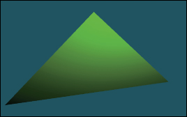
Figure 15.7: A green Lambertian triangle.
15.4.7. Glossy Scattering
The Lambertian surface appears dull because it has no highlight. A common approach for producing a more interesting shiny surface is to model it with something like the Blinn-Phong scattering function. An implementation of this function with the energy conservation factor from Sloan and Hoffmann [AMHH08, 257] is given in Listing 15.19. See Chapter 27 for a discussion of the origin of this function and alternatives to it. This is a variation on the shading function that we saw back in Chapter 6 in WPF, only now we are implementing it instead of just adjusting the parameters on a black box. The basic idea is simple: Extend the Lambertian BSDF with a large radial peak when the normal lies close to halfway between the incoming and outgoing directions. This peak is modeled by a cosine raised to a power since that is easy to compute with dot products. It is scaled so that the outgoing radiance never exceeds the incoming radiance and so that the sharpness and total intensity of the peak are largely independent parameters.
Listing 15.19: Blinn-Phong BSDF scattering density.
1classBSDF{ 2public: 3Color3k_L; 4Color3k_G; 5floats; 6Vector3n; 7 . . . 8 9Color3evaluateFiniteScatteringDensity(constVector3& w_i, 10constVector3& w_o)const{ 11constVector3& w_h = (w_i + w_o).direction(); 12return13 (k_L + k_G * ((s + 8.0f) * 14 powf(std::max(0.0f, w_h.dot(n)), s) / 8.0f)) / 15 PI; 16 17 } 18 };
For this BSDF, choose lambertian + glossy < 1 at each color channel to ensure energy conservation, and glossySharpness typically in the range [0, 2000]. The glossySharpness is on a logarithmic scale, so it must be moved in larger increments as it becomes larger to have the same perceptual impact.
Figure 15.8 shows the green triangle rendered with the normalized Blinn-Phong BSDF. Here, k_L=Color3(0.0f, 0.0f, 0.8f), k_G=Color3(0.2f, 0.2f, 0.2f), and s=100.0f.
)
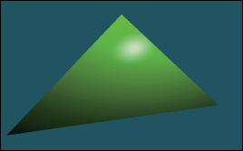
Figure 15.8: Triangle rendered with a normalized Blinn-Phong BSDF.
15.4.8. Shadows
The shade function in Listing 15.17 only adds the illumination contribution from a light source if there is an unoccluded line of sight between that source and the point P being shaded. Areas that are occluded are therefore darker. This absence of light is the phenomenon that we recognize as a shadow.
In our implementation, the line-of-sight visibility test is performed by the visible function, which is supposed to return true if and only if there is an unoccluded line of sight. While working on the shading routine we temporarily implemented visible to always return true, which means that our images contain no shadows. We now revisit the visible function in order to implement shadows.
We already have a powerful tool for evaluating line of sight: the intersect function. The light source is not visible from P if there is some intersection with another triangle. So we can test visibility simply by iterating over the scene again, this time using the shadow ray from P to the light instead of from the camera to P. Of course, we could also test rays from the light to P.
Listing 15.20 shows the implementation of visible. The structure is very similar to that of sampleRayTriangle. It has three major differences in the details. First, instead of shading the intersection, if we find any intersection we immediately return false for the visibility test. Second, instead of casting rays an infinite distance, we terminate when they have passed the light source. That is because we don’t care about triangles past the light—they could not possibly cast shadows on P. Third and finally, we don’t really start our shadow ray cast at P. Instead, we offset it slightly along the ray direction. This prevents the ray from reintersecting the surface containing P as soon as it is cast.
Listing 15.20: Line-of-sight visibility test, to be applied to shadow determination.
1boolvisible(constVector3& P,constVector3& direction,floatdistance,constScene& scene){ 2static const floatrayBumpEpsilon = 1e-4; 3constRay shadowRay(P + direction * rayBumpEpsilon, direction); 4 5 distance -= rayBumpEpsilon; 6 7// Test each potential shadow caster to see if it lies between P and the light8floatignore[3]; 9for(unsigned ints = 0; s < scene.triangleArray.size(); ++s) { 10if(intersect(shadowRay, scene.triangleArray[s], ignore) < distance) { 11// This triangle is closer than the light12return false; 13 } 14 } 15 16return true; 17 }
Our single-triangle scene is insufficient for testing shadows. We require one object to cast shadows and another to receive them. A simple extension is to add a quadrilateral “ground plane” onto which the green triangle will cast its shadow. Listing 15.21 gives code to create this scene. Note that this code also adds another triangle with the same vertices as the green one but the opposite winding order. Because our triangles are single-sided, the green triangle would not cast a shadow. We need to add the back of that surface, which will occlude the rays cast upward toward the light from the ground.
Figure 15.9 shows how the new scene should render before you implement shadows. If you do not see the ground plane under your own implementation, the most likely error is that you failed to loop over all triangles in one of the ray-casting routines.
)
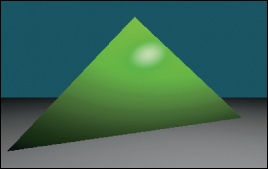
Figure 15.9: The green triangle scene extended with a two-triangle gray ground “plane.” A back surface has also been added to the green triangle.
Listing 15.21: Scene-creation code for a two-sided triangle and a ground plane.
1voidmakeOneTriangleScene(Scene& s) { s.triangleArray.resize(1); 2 3 s.triangleArray[0] = 4Triangle(Vector3(0,1,-2),Vector3(-1.9,-1,-2),Vector3(1.6,-0.5,-2), 5Vector3(0,0.6f,1).direction(), 6Vector3(-0.4f,-0.4f, 1.0f).direction(), 7Vector3(0.4f,-0.4f, 1.0f).direction(), 8BSDF(Color3::green() * 0.8f,Color3::white() * 0.2f, 100)); 9 10 s.lightArray.resize(1); 11 s.lightArray[0].position =Point3(1, 3, 1); 12 s.lightArray[0].power =Color3::white() * 10.0f; 13 } 14 15voidmakeTrianglePlusGroundScene(Scene& s) { 16 makeOneTriangleScene(s); 17 18// Invert the winding of the triangle19 s.triangleArray.push_back 20 (Triangle(Vector3(-1.9,-1,-2),Vector3(0,1,-2), 21Vector3(1.6,-0.5,-2),Vector3(-0.4f,-0.4f, 1.0f).direction(), 22Vector3(0,0.6f,1).direction(),Vector3(0.4f,-0.4f, 1.0f).direction(), 23BSDF(Color3::green() * 0.8f,Color3::white() * 0.2f, 100))); 24 25// Ground plane26const floatgroundY = -1.0f; 27constColor3groundColor =Color3::white() * 0.8f; 28 s.triangleArray.push_back 29 (Triangle(Vector3(-10, groundY, -10),Vector3(-10, groundY, -0.01f), 30Vector3(10, groundY, -0.01f), 31Vector3::unitY(),Vector3::unitY(),Vector3::unitY(), groundColor)); 32 33 s.triangleArray.push_back 34 (Triangle(Vector3(-10, groundY, -10),Vector3(10, groundY, -0.01f), 35Vector3(10, groundY, -10), 36Vector3::unitY(),Vector3::unitY(),Vector3::unitY(), groundColor)); 37 }
Figure 15.10 shows the scene rendered with visible implemented correctly. If the rayBumpEpsilon is too small, then shadow acne will appear on the green triangle. This artifact is shown in Figure 15.11. An alternative to starting the ray artificially far from P is to explicitly exclude the previous triangle from the shadow ray intersection computation. We chose not to do that because, while appropriate for unstructured triangles, it would be limiting to maintain that custom ray intersection code as our scene became more complicated. For example, we would like to later abstract the scene data structure from a simple array of triangles. The abstract data structure might internally employ a hash table or tree and have complex methods. Pushing the notion of excluding a surface into such a data structure could complicate that data structure and compromise its general-purpose use. Furthermore, although we are rendering only triangles now, we might wish to render other primitives in the future, such as spheres or implicit surfaces. Such primitives can intersect a ray multiple times. If we assume that the shadow ray never intersects the current surface, those objects would never self-shadow.
)
)

Figure 15.10: A four-triangle scene, with ray-cast shadows implemented via the visible function. The green triangle is two-sided.
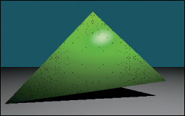
Figure 15.11: The dark dots on the green triangle are shadow acne caused by self-shadowing. This artifact occurs when the shadow ray immediately intersects the triangle that was being shaded.
15.4.9. A More Complex Scene
Now that we’ve built a renderer for one or two triangles, it is no more difficult to render scenes containing many triangles. Figure 15.12 shows a shiny, gold-colored teapot on a white ground plane. We parsed a file containing the vertices of the corresponding triangle mesh, appended those triangles to the Scene’s triangle array, and then ran the existing renderer on it. This scene contains about 100 triangles, so it renders about 100 times slower than the single-triangle scene. We can make arbitrarily more complex geometry and shading functions for the renderer. We are only limited by the quality of our models and our rendering performance, both of which will be improved in subsequent chapters.
)
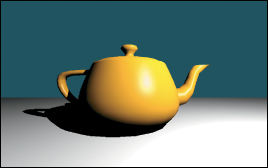
Figure 15.12: A scene composed of many triangles.
This scene looks impressive (at least, relative to the single triangle) for two reasons. First, we see some real-world phenomena, such as shiny highlights, shadows, and nice gradients as light falls off. These occurred naturally from following the geometric relationships between light and surfaces in our implementation.
Second, the image resembles a recognizable object, specifically, a teapot. Unlike the illumination phenomena, nothing in our code made this look like a teapot. We simply loaded a triangle list from a data file that someone (originally, Jim Blinn) happened to have manually constructed. This teapot triangle list is a classic model in graphics. You can download the triangle mesh version used here from http://graphics.cs.williams.edu/data among other sources. Creating models like this is a separate problem from rendering, discussed in Chapter 22 and many others. Fortunately, there are many such models available, so we can defer the modeling problem while we discuss rendering.
We can learn a lesson from this. A strength and weakness of computer graphics as a technical field is that often the data contributes more to the quality of the final image than the algorithm. The same algorithm rendered the teapot and the green triangle, but the teapot looks more impressive because the data is better. Often a truly poor approximation algorithm will produce stunning results when a master artist creates the input—the commercial success of the film and game industries has largely depended on this fact. Be aware of this when judging algorithms based on rendered results, and take advantage of it by importing good artwork to demonstrate your own algorithms.