Cluster Analysis in Excel

This chapter is from the book

Statistical Analysis: Microsoft Excel 2016

Learn More Buy

This chapter is from the book

This chapter is from the book 

Statistical Analysis: Microsoft Excel 2016

Learn More Buy

Calculating the Mode

The mean gives you a measure of central tendency by taking all the actual values in a group into account. The median measures central tendency differently, by giving you the midpoint of a ranked group of values. The mode takes yet another tack: It tells you which one of several values occurs most frequently.

You can get this information from the FREQUENCY() function, as discussed in Chapter 1. But the MODE() function returns the most frequently occurring observation only, and it’s a little quicker to use than FREQUENCY() is. Furthermore, as you’ll see in this section, a little work can get MODE() to work with data on a nominal scale—that’s also possible with FREQUENCY(), but it’s a lot more work.

Suppose you have a set of numbers in a range of cells, as shown in Figure 2.8. The following formula returns the numeric value that occurs most frequently in that range (in Figure 2.8, the formula is entered in cell C1):

=MODE(A2:A21)

Figure 2.8

Excel’s MODE() function works only with numeric values.

The pivot chart in Figure 2.8 provides the same information graphically. Notice that the mode returned by the function in cell C1 is the same value as the most frequently occurring value shown in the pivot chart.

The problem is that you don’t usually care about the mode of numeric values. It’s possible that you have at hand a list of the ages of the people who live on your block, or the weight of each player on your favorite football team, or the height of each student in your daughter’s fourth grade class. It’s even conceivable that you have a good reason to know the most frequently occurring age, weight, or height in a group of people. (In the area of inferential statistics, covered in the second half of this book, the mode of what’s called a reference distribution is often of interest. At this point, though, we’re dealing with more commonplace problems.) But you don’t normally need the mode of people’s heights, of irises’ sepal lengths, or the ages of rocks.

Among other purposes, numeric measures are good for recording small distinctions: Joe is 33 years old and Jane is 34; Dave weighs 230 pounds and Don weighs 232; Jake is 47 inches tall and Judy stands 48 inches. In a group of 18 or 20 people, it’s quite possible that everyone is of a different age, or a different weight or a different height. The same is true of most objects and numeric measurements that you can think of.

In that case, it is not plausible that you would want to know the modal age, or weight, or height. The mean, yes, or the median, but why would you want to know that the most frequently occurring age in your poker club is 47 years, when the next most frequently occurring age is 46 and the next is 48?

The mode is seldom a useful statistic when the variable being studied is numeric and ungrouped. It’s when you are interested in nominal data—as discussed in Chapter 1, categories such as brands of cars or children’s given names or political preferences—that the mode is of interest. It’s worth noting that the mode is the only sensible measure of central tendency when you’re dealing with nominal data. The modal boy’s name for newborns in 2015 was Noah; that statistic is interesting to some people in some way. But what’s the mean of Jacob, Michael, and Ethan? The median of Emma, Isabella, and Emily? The mode is the only sensible measure of central tendency for nominal data.

But Excel’s MODE() function doesn’t work with nominal data. If you present to it, as its argument, a range that contains exclusively text data such as names, MODE() returns the #N/A error value. If one or more text values are included in a list of numeric values, MODE() simply ignores the text values.

I’ll take this opportunity to complain that it doesn’t make a lot of sense for Excel to provide analytic support for a situation that seldom occurs (for example, caring about the modal height of a group of fourth graders) while it fails to support situations that occur all the time (“Which model of car did we sell most of last week?”).

Figure 2.9 shows a couple of solutions to the problem with MODE().

Figure 2.9

MODE() is much more useful with categories than with interval or ordinal scales of measurement.

The frequency distribution in Figure 2.9 is more informative than the pivot chart shown in Figure 2.8, where just one value pokes up above the others because it occurs twice instead of once. You can see that Ford, the modal value, leads Toyota by a slim margin and GM by somewhat more. (This report is genuine and was exported to Excel by a used car dealer from a popular small business accounting package.)

To create a pivot chart that looks like the one in Figure 2.9, follow these steps:

1. Arrange your raw data in an Excel list format: the field name in the first column (such as A1) and the values in the cells below the field name (such as A2:A21). It’s best if all the cells immediately adjacent to the list are empty.
2. Select a cell in your list.
3. Click the Ribbon’s Insert tab, and click the PivotChart button in the Charts group. The dialog box shown in Figure 2.10 appears.
   

   Figure 2.10

   In this dialog box you can accept or edit the location of the underlying data, and indicate where you want to pivot table to start.

   
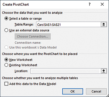
4. If you took step 2 and selected a cell in your list before clicking the PivotChart button, Excel has automatically supplied the list’s address in the Table/Range edit box. Otherwise, identify the range that contains your raw data by dragging through it with your mouse pointer, by typing its range address, or by typing its name if it’s a named table or range. The location of the data should now appear in the Table/Range edit box.
5. If you want the pivot table and pivot chart to appear in the active worksheet, click the Existing Worksheet button and click in the Location edit box. Then click in a worksheet cell that has several empty columns to its right and several empty rows below it. This is to keep Excel from asking if you want the pivot table to overwrite existing data. Click OK to get the layout shown in Figure 2.11.
   

   Figure 2.11

   The PivotChart Field pane appears automatically.

   
6. In the PivotChart Fields pane, drag the field or fields you’re interested in down from the list and into the appropriate area at the bottom. In this example, you would drag Make down into the Axis (Categories) area and also drag it into the Σ Values area.

The pivot chart and the pivot table that the pivot chart is based on both update as soon as you’ve dropped a field into an area in the PivotTable Fields pane. If you started with the data shown in Figure 2.9, you should get a pivot chart that’s identical, or nearly so, to the pivot chart in that figure.

A few comments on this analysis:

• The mode is quite a useful statistic when it’s applied to categories: political parties, consumer brands, days of the week, states in a region, and so on. Excel really should have a built-in worksheet function that returns the mode for text values. But it doesn’t, and the next section shows you how to write your own worksheet formula for the mode, one that will work for both numeric and text values.
• When you have just a few distinct categories, consider building a pivot chart to show how many instances there are of each. A pivot chart that shows the number of instances of each category is an appealing way to present your data to an audience. (There is no type of chart that communicates well when there are many categories to consider. The visual clutter obscures the message. In that sort of situation, consider combining categories or omitting some.)
• Standard Excel charts do not show the number of instances per category without some preliminary work. You would have to get a count of each category before creating the chart, and that’s the purpose of the pivot table that underlies the pivot chart. The pivot chart, based on the pivot table, is simply a faster way to complete the analysis than creating your own table to count category membership and then basing a standard Excel chart on that table.
• The mode is the only sensible measure of central tendency when you’re working with nominal data such as category names. The median requires that you rank order things in some way: shortest to tallest, least expensive to priciest, or slowest to fastest. In terms of the scale types introduced in Chapter 1, you need at least an ordinal scale to get a median, and many categories are nominal, not ordinal. Variables that are represented by values such as Ford, GM, and Toyota have neither a mean nor a median.

Getting the Mode of Categories with a Formula

I have pointed out that Excel’s MODE() function does not work when you supply it with text values as its arguments. Here is a method for getting the mode using a worksheet formula. It tells you which text value occurs most often in your data set. You’ll also see how to enter a formula that tells you how many instances of the mode exist in your data.

If you don’t want to resort to a pivot chart to get the mode of a group of text values, you can get their mode with the formula

=INDEX(A2:A21,MODE(MATCH(A2:A21,A2:A21,0)))

assuming that the text values are in A2:A21. (The range could occupy a single column, as in A2:A21, or a single row, as in A2:Z2. It will not work properly with a multirow, multicolumn range such as A2:Z21.)

If you’re somewhat new to Excel, that formula isn’t going to make any sense to you at all. I structured it, I’ve been using Excel frequently since 1994, and I still have to stare at the formula and think it through before I see why it returns the mode. So if the formula seems baffling, don’t worry about it. It will become clear in the fullness of time, and in the meantime you can use it to get the modal value for any set of text values in a worksheet. Simply replace the range address A2:A21 with the address of the range that contains your text values.

Briefly, the components of the formula work as follows:

• The MATCH() function returns the position in the array of values where each individual value first appears. The third argument to the MATCH() function, 0, tells Excel that in each case an exact match is required and the array is not necessarily sorted. So, for each instance of Ford in the array of values in A2:A21, MATCH() returns 1; for each instance of Toyota, it returns 2; for each instance of GM, it returns 4.
• The results of the MATCH() function are used as the argument to MODE(). In this example, there are 20 values for MODE() to evaluate: some equal 1, some equal 2, and some equal 4. MODE() returns the most frequently occurring of those numbers.
• The result of MODE() is used as the second argument to INDEX(). Its first argument is the array to examine. The second argument tells it how far into the array to look. Here, it looks at the first value in the array, which is Ford. If, say, GM had been the most frequently occurring text value, MODE() would have returned 4 and INDEX() would have used that value to find GM in the array.

Using an Array Formula to Count the Values

With the modal value (Ford, in this example) in hand, we still want to know how many instances there are of that mode. This section describes how to create the array formula that counts the instances.

Figure 2.9 also shows, in cell C2, the count of the number of records that belong to the modal value. This formula provides that count:

=SUM(IF(A2:A21=C1,1,0))

The formula is an array formula, and must be entered using the special keyboard sequence Ctrl+Shift+Enter. You can tell that a formula has been entered as an array formula if you see curly brackets around it in the formula box. If you array-enter the prior formula, it looks like this in the formula box:

{=SUM(IF(A2:A21=C1,1,0))}

But don’t supply the curly brackets yourself. If you do, Excel interprets this as text, not as a formula.

Here’s how the formula works: As shown in Figure 2.9, cell C1 contains the value Ford. So the following fragment of the array formula tests whether values in the range A2:A21 equal the value Ford:

A2:A21=C1

Because there are 20 cells in the range A2:A21, the fragment returns an array of TRUE and FALSE values: TRUE when a cell contains Ford and FALSE otherwise. The array looks like this:

{TRUE;FALSE;TRUE;FALSE;FALSE;FALSE;TRUE;FALSE;TRUE;TRUE;FALSE;FALSE;FALSE;TRUE;TRUE;FALSE;FALSE;TRUE;FALSE;FALSE}

Specifically, cell A2 contains Ford, and so it passes the test: The first value in the array is therefore TRUE. Cell A3 does not contain Ford, and so it fails the test: The second value in the array is therefore FALSE—and so on for all 20 cells.

Now step outside that fragment, which, as we’ve just seen, resolves to an array of TRUE and FALSE values. The array is used as the first argument to the IF() function. Excel’s IF() function takes three arguments:

• The first argument is a value that can be TRUE or FALSE. In this example, that’s each value in the array just shown, returned by the fragment A2:A21=C1.
• The second argument is the value that you want the IF() function to return when the first argument is TRUE. In the example, this is 1.
• The third argument is the value that you want the IF() function to return when the first argument is FALSE. In the example, this is 0.

The IF() function examines each of the values in the array to see if it’s a TRUE value or a FALSE value. When a value in the array is TRUE, the IF() function returns, in this example, a 1, and a 0 otherwise. Therefore, the fragment

IF(A2:A21=C1,1,0)

returns an array of 1s and 0s that corresponds to the first array of TRUE and FALSE values. That array looks like this:

{1;0;1;0;0;0;1;0;1;1;0;0;0;1;1;0;0;1;0;0}

A 1 corresponds to a cell in A2:A21 that contains the value Ford, and a 0 corresponds to a cell in the same range that does not contain Ford. Finally, the array of 1s and 0s is presented to the SUM() function, which totals the values in the array. Here, that total is 8.

Recapping the Array Formula

To review how the array formula counts the values for the modal category of Ford, consider the following:

• The formula’s purpose is to count the number of instances of the modal category, Ford, whose name is in cell C1.
• The innermost fragment in the formula, A2:A21=C1, returns an array of 20 TRUE or FALSE values, depending on whether each of the 20 cells in A2:A21 contains the same value as is found in cell C1.
• The IF() function examines the TRUE/FALSE array and returns another array that contains 1s where the TRUE/FALSE array contains TRUE, and 0s where the TRUE/FALSE array contains FALSE.
• The SUM() function totals the values in the array of 1s and 0s. The result is the number of cells in A2:A21 that contain the value in cell C1, which is the modal value for A2:A21.

Using an Array Formula

Various reasons exist for using array formulas in Excel. Two of the most typical reasons are to support a function that requires it be array-entered, and to enable a function to work on more than just one value.

Accommodating a Function 

One reason you might need to use an array formula is that you’re employing a function that must be array-entered if it is to return results properly. For example, the FREQUENCY() function, which counts the number of values between a lower bound and an upper bound (see “Defining Arguments,” earlier in this chapter) requires that you enter it in an array formula. Another function that requires array entry is the LINEST() function, which will be discussed in great detail in several subsequent chapters.

Both FREQUENCY() and LINEST(), along with a number of other functions, return an array of values to the worksheet. You need to accommodate that array. To do so, begin by selecting a range of cells that has the number of rows and columns needed to show the function’s results. (Knowing how many rows and columns to select depends on your knowledge of the function and your experience with it.) Then you enter the formula that calls the function by means of Ctrl+Shift+Enter instead of simply Enter; again, this sequence is called array-entering the formula.

Accommodating a Function’s Arguments 

Sometimes you use an array formula because it employs a function that usually takes a single value as an argument, but you want to supply it with an array of values. The example in cell C2 of Figure 2.9 shows the IF() function, which usually expects a single condition as its first argument, instead accepting an array of TRUE and FALSE values as its first argument:{59}

=SUM(IF(A2:A21=C1,1,0))

Typically, the IF() function deals with only one value in its first argument. For example, suppose you want cell C2 to show the value Current if cell A1 contains the value 2018; otherwise, B1 should show the value Past. You could put this formula in B1, entered normally with the Enter key:

If you’re using Excel 2002 or a more recent version, you have access to a formula evaluation tool. Begin by selecting a cell that contains a formula. Then start formula evaluation. In Excel 2007 through 2016, you’ll find it on the Ribbon’s Formulas tab, in the Formula Auditing group; in Excel 2002 and 2003, choose Tools, Formula Auditing, Evaluate Formula. If you were to begin by selecting a cell with the array formula that this section has discussed, you would see the window shown in Figure 2.12.

Figure 2.12

Formula evaluation starts with the formula as it’s entered in the active cell.

Now, if you click Evaluate, Excel begins evaluating the formula from the inside out, and the display changes to what you see in Figure 2.13.

Figure 2.13

The formula expands to show the contents of A2:A21 and C1.

Click Evaluate again and you see the results of the test of A2:A21 with C1, as shown in Figure 2.14.

Figure 2.14

The array of cell contents becomes an array of TRUE and FALSE, depending on the contents of the cells.

Click Evaluate again and the window shows the results of the IF() function, which in this case replaces TRUE with 1 and FALSE with 0 (see Figure 2.15).

Figure 2.15

Each 1 represents a cell that equals the value in cell C1.

A final click of Evaluate shows you the final result, when the SUM() function totals the 1s and 0s to return a count of the number of instances of Ford in A2:A21, as shown in Figure 2.16.

Figure 2.16

There are eight instances of Ford in A2:A21.

You could use the SUMIF() or COUNTIF() function if you prefer. I like the SUM(IF()) structure because I find that it gives me more flexibility in complicated situations such as summing the results of multiplying two or more conditional arrays.

Using the Recalculate Key 

Another method for looking inside a formula is available in all Windows versions of Excel, and makes use of the F9 key. The F9 key forces a calculation and can be used to recalculate a worksheet’s formulas when automatic recalculation has been turned off.

If that were all you could do with the F9 key, its scope would be pretty limited. But you can also use it to calculate a portion of a formula. Suppose that you have this array formula in a worksheet cell and its arguments as given in Figure 2.9:

=SUM(IF(A2:A21=C1,1,0))

If the cell that contains the formula is active, you’ll see the formula in the formula box. Drag across the A2:A21=C1 portion with your mouse pointer to highlight it. Then, while it’s still highlighted, press F9 to get the result shown in Figure 2.17, in the formula bar.

Figure 2.17

Notice that the array of TRUE and FALSE values is identical to the one shown in Figure 2.14.

Excel formulas separate rows by semicolons and columns by commas. The array in Figure 2.17 is based on values that are found in different rows, so the TRUE and FALSE items are separated by semicolons. If the original values were in different columns, the TRUE and FALSE items would be separated by commas.

If you’re using Excel 2002 or later, use formula evaluation to step through a formula from the inside out. Alternatively, using any Windows version of Excel, use the F9 key to get a quick look at how Excel evaluates a single fragment from the formula.