Using Regression to Test Differences Between Group Means
Analysis expert Conrad Carlberg discusses the use of regression analysis to analyze the influence of nominal variables (such as make of car or type of medical treatment) on interval variables (such as gas mileage or levels of indicators in blood tests).
This is a book about regression analysis. Nevertheless, I’m going to start this chapter by discussing different scales of measurement. When you use regression analysis, your predicted (or outcome, or dependent) variable is nearly always measured on an interval or ratio scale, one whose values are numeric quantities. Your predictor (or independent, or regressor) variables are also frequently measured on such numeric scales.
However, the predictor variables can also represent nominal or category scales. Because functions such as Excel’s LINEST() do not respond directly to predictors with values such as STATIN and PLACEBO, or REPUBLICAN and DEMOCRAT, you need a system to convert those nominal values to numeric values that LINEST() can deal with.
The system you choose has major implications for the information you get back from the analysis. So I’ll be taking a closer look at some of the underlying issues that inform your choice.
It will also be helpful to cover some terminology issues early on. This book’s first six chapters have discussed the use of regression analysis to assess the relationships between variables measured on an interval or a ratio scale. There are a couple of reasons for that:
Discussing interval variables only allows us to wait until now to introduce the slightly greater complexity of using regression to assess differences between groups.
Most people who have heard of regression analysis at all have heard of it in connection with prediction and explanation: for example, predicting weight from known height. That sort of usage tends to imply interval or ratio variables as both the predicted variable and the predictor variables.
With this chapter we move into the use of regression analysis to analyze the influence of nominal variables (such as make of car or type of medical treatment) on interval variables (such as gas mileage or levels of indicators in blood tests). That sort of assessment tends to focus on the effects of belonging to different groups upon variables that quantify the outcome of group membership (gas mileage for different auto makes or cholesterol levels after different medical treatments).
We get back to the effects of interval variables in Chapter 8, “The Analysis of Covariance,” but in this chapter I’ll start referring to what earlier chapters called predicted variables as outcome variables, and what I have called predictor variables as factors. Lots of theorists and writers prefer terms other than outcome variable, because it implies a cause-and-effect relationship, and inferring that sort of situation is a job for your experimental design, not your statistical analysis. But as long as that’s understood, I think we can get along with outcome variable—at least, it’s less pretentious than some of its alternatives.
Dummy Coding
Perhaps the simplest approach to coding a nominal variable is termed dummy coding. I don’t mean the word “simplest” to suggest that the approach is underpowered or simple-minded. For example, I prefer dummy coding in logistic regression, where it can clarify the interpretation of the coefficients used in that method.
Dummy coding can also be useful in standard linear regression when you want to compare one or more treatment groups with a comparison or control group.
An Example with Dummy Coding
Figures 7.1 and 7.2 show how the data from a small experiment could be set up for analysis by an application that returns a traditional analysis of variance, or ANOVA.
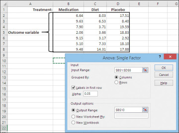
Figure 7.1 The Data Analysis tool requires that the factor levels occupy different columns or different rows.
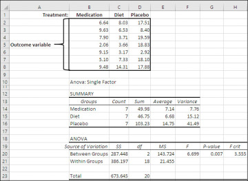
Figure 7.2 If you choose Labels in First Row in the dialog box, the output associates the summary statistics with the label.
In ANOVA jargon, a variable whose values constitute the different conditions to which the subjects are exposed is called a factor. In this example, the factor is Treatment. The different values that the Treatment factor can take on are called levels. Here, the levels are the three treatments: Medication, Diet, and Placebo as a means of lowering amounts of an undesirable component in the blood.
Excel’s Data Analysis add-in includes a tool named ANOVA: Single Factor. To operate correctly, the data set must be arranged as in the range B2:C8 of Figure 7.2. (Or it may be turned 90 degrees, to have different factor levels in different rows and different subjects in different columns.) With the data laid out as shown in the figure, you can run the ANOVA: Single Factor tool and in short order get back the results shown in the range A12:H23. The Data Analysis tool helpfully provides descriptive statistics as shown in B14:F16.
Figure 7.3 has an example of how you might use dummy coding to set up an analysis of the same data set by means of regression analysis via dummy coding.
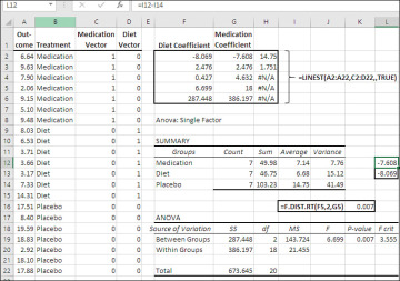
Figure 7.3 One minor reason to prefer the regression approach is that you use standard Excel layouts for the data.
When you use any sort of coding there are a couple of rules to follow. These are the rules that apply to dummy coding:
You need to reserve as many columns for new data as the factor has levels, minus 1. Notice that this is the same as the number of degrees of freedom for the factor. With three levels, as in the present example, that’s 3 − 1, or 2. It’s useful to term these columns vectors.
Each vector represents one level of the factor. In Figure 7.3, Vector 1 represents Medication, so every subject who receives the medication gets a 1 on Vector 1, and everyone else receives a 0 on that vector. Similarly, every subject receives a 0 on Vector 2 except those who are treated by Diet—they get a 1 on Vector 2.
Subjects in one level, which is often a control group, receive a 0 on all vectors. In Figure 7.3, this is the case for those who take a placebo.
With the data laid out as shown in the range A2:D22 in Figure 7.3, array-enter this LINEST() function in a blank range five rows high and three columns wide, such as F2:H6 in the figure:
=LINEST(A2:A22,C2:D22,,TRUE)
Don’t forget to array-enter the formula with the keyboard combination Ctrl+Shift+Enter. The arguments are as follows:
The first argument, the range A2:A22, is the address that contains the outcome variable. (Because the description of this study suggests that it’s a true, controlled experiment, it’s not misleading to refer to the levels of a given component in the blood as an outcome variable, thus implying cause and effect.)
The second argument, the range C2:D22, is the address that contains the vectors that indicate which level of the factor a subject belongs to. In other experimental contexts you might refer to these as predictor variables.
The third argument is omitted, as indicated by the consecutive commas with nothing between them. If this argument is TRUE or omitted, Excel is instructed to calculate the regression equation’s constant normally. If the argument is FALSE, Excel is instructed to set the constant to 0.0.
The fourth argument, TRUE, instructs Excel to calculate and return the third through fifth rows of the results, which contain summary information, mostly about the reliability of the regression equation.
In Figure 7.3 I have repeated the results of the traditional ANOVA from Figure 7.2, to make it easier to compare the results of the two analyses. Note these points:
The sum of squares regression and the sum of squares residual from the LINEST() results in cells F6 and G6 are identical to the sum of squares between groups and the sum of squares within groups returned by the Data Analysis add-in in cells G19 and G20.
The degrees of freedom for the residual in cell G5 is the same as the degrees of freedom within groups in cell H20. Along with the sums of squares and knowledge of the number of factor levels, this enables you to calculate the mean square between and the mean square within if you want.
The F-ratio returned in cell F5 by LINEST() is identical to the F-ratio reported by the Data Analysis add-in in cell J19.
The constant (also termed the intercept) returned by LINEST() in cell H2 is identical to the mean of the group that’s assigned codes of 0 throughout the vectors. In this case that’s the Placebo group: Compare the value of the constant in cell H2 with the mean of the Placebo group in cell I14. (That the constant equals the group with codes of 0 throughout is true of dummy coding, not effect or orthogonal coding, discussed later in this chapter.)
The regression coefficients in cells F2 and G2, like the t-tests in Chapter 6, express the differences between group means. In the case of dummy coding, the difference is between the group assigned a code of 1 in a vector and the group assigned 0’s throughout.
For example, the difference between the means of the group that took a medication and the group that was treated by placebo is 7.14 − 14.75 (see cells I12 and I14). That difference equals −7.608, and it’s calculated in cell L12. That’s the regression coefficient for Vector 1, returned by LINEST() in cell G2. Vector 1 identifies the Medication group with a 1.
Similarly, the difference between the mean of the group treated by diet and that treated by placebo is 6.68 − 14.75 (see cells I13 and I14). The difference equals −8.069, calculated in cell L13, which is also the regression coefficient for Vector 2.
One bit of information that LINEST() does not provide you is statistical significance of the regression equation. In the context of ANOVA, where we’re evaluating the differences between group means, that test of statistical significance asks whether any of the mean differences is large enough that the null hypothesis of no difference between the means in the population can be rejected. The F-ratio, in concert with the degrees of freedom for the regression and the residual, speaks to that question.
You can determine the probability of observing a given F-ratio if the null hypothesis is true by using Excel’s F.DIST.RT() function. In this case, you use it in this way (it’s also in cell K16):
=F.DIST.RT(F5,2,G5)
Notice that the value it returns, 0.007, is identical to that returned in cell K19 by the Data Analysis add-in’s ANOVA: Single Factor tool. If there is no difference, measured by group means, in the populations of patients who receive the medication, or whose diet was controlled, or who took a placebo, then the chance of observing an F-ratio of 6.699 is 7 in 1,000. It’s up to you whether that’s rare enough to reject the null hypothesis. It would be for most people, but a sample of 21 is a very small sample, and that tends to inhibit the generalizability of the findings—that is, how confidently you can generalize your observed outcome from 21 patients to your entire target population.
Populating the Vectors Automatically
So: What does all this buy you? Is there enough advantage to running your ANOVA using regression in general and LINEST() in particular that it justifies any extra work involved?
I think it does, and the decision isn’t close. First, what are the steps needed to prepare for the Data Analysis tool, and what steps to prepare a regression analysis?
To run the Data Analysis ANOVA: Single Factor tool, you have to arrange your data as shown in the range B1:D8 in Figure 7.2. That’s not a natural sort of arrangement of data in either a true database or in Excel. A list or table structure of the sort shown in A1:D22 of Figure 7.3 is much more typical, and as long as you provide columns C and D for the dummy 0/1 codes, it’s ready for you to point LINEST() at.
To prepare for a regression analysis, you do need to supply the 0s and 1s in the proper rows and the proper columns. This is not a matter of manually entering 0s and 1s one by one. Nor is it a matter of copying and pasting values or using Ctrl+Enter on a multiple selection. I believe that the fastest, and most accurate, way of populating the coded vectors is by way of Excel’s VLOOKUP() function. See Figure 7.4.
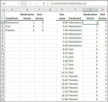
Figure 7.4 Practice in the use of the VLOOKUP() function can save you considerable time in the long run.
To prepare the ground, enter a key such as the one in the range A2:C4 in Figure 7.4. That key should have as many columns and as many rows as the factor has levels. In this case, the factor has three levels (Medication, Diet, and Placebo), so the key has three columns, and there’s one row for each level. It’s helpful but not strictly necessary to provide column headers, as is done in the range A1:C1 of Figure 7.4.
The first column—in this case, A2:A4—should contain the labels you use to identify the different levels of the factor. In this case those levels are shown for each subject in the range F2:F22.
You can save a little time by selecting the range cells in the key starting with its first row and its second column—so, B2:C4. Type 0, hold down the Ctrl key and press Enter. All the selected cells will now contain the value 0.
In the same row as a level’s label, enter a 1 in the column that will represent that level. So, in Figure 7.4, cell B2 gets a 1 because column B represents the Medication level, and cell C3 gets a 1 because column C represents the Diet level. There will be no 1 to represent Placebo because we’ll treat that as a control or comparison group, and so it gets a 0 in each column.
With the key established as in A2:C4 of Figure 7.4, select the first row of the first column where you want to establish your matrix of 0’s and 1’s. In Figure 7.4, that’s cell G2. Enter this formula:
=VLOOKUP($F2,$A$2:$C$4,2,0)
Where:
$F2 is the label that you want to represent with a 1 or a 0.
$A$2:$C$4 contains the key (Excel terms this a table lookup).
2 identifies the column in the key that you want returned.
0 specifies that an exact match for the label is required, and that the labels in the first column of the key are not necessarily sorted.
I’ve supplied dollar signs where needed in the formula so that it can be copied to other columns and rows without disrupting the reference to the key’s address, and to the column in which the level labels are found.
Now copy and paste cell G2 into H2 (or use the cell’s selection handle to drag it one column right). In cell H2, edit the formula so that VLOOKUP()’s third argument has a 3 instead of a 2—this directs Excel to look in the key’s third column for its value.
Finally, make a multiple selection of cells G2 and H2, and drag them down into G3:H22. This will populate columns G and H with the 0’s and 1’s that specify which factor level each record belongs to.
You can now obtain the full LINEST() analysis by selecting a range such as A6:C10, and array-entering this formula:
=LINEST(E2:E22,G2:H22,,TRUE)
By the way, you might find it more convenient to switch the contents of columns E and F in Figure 7.4. I placed the treatment labels in column F to ease the comparison of the labels with the dummy codes. If you swap columns E and F, you might find the LINEST() -formula easier to handle. You’ll also want to change the first VLOOKUP() formula from this:
=VLOOKUP($F2,$A$2:$C$4,2,0)
to this:
=VLOOKUP($E2,$A$2:$C$4,2,0)
The Dunnett Multiple Comparison Procedure
When you have completed a test of the differences between the means of three or more groups—whether by way of traditional ANOVA methods or a regression approach—you have learned the probability that any of the means in the population is different from any of the remaining means in the population. You have not learned which mean or means is different from others.
Statisticians studied this issue and wrote an intimidatingly comprehensive literature on the topic during the middle years of the twentieth century. The procedures they developed came to be known as multiple comparisons. Depending on how you count them, the list of different procedures runs to roughly ten. The procedures differ from one another in several ways, including the nature of the error involved (for example, per comparison or per experiment), the reference distribution (for example, F, t, or q), planned beforehand (a priori) or after the fact (post hoc), and on other dimensions.
If you choose to use dummy coding in a regression analysis, in preference to another coding method, it might well be because you want to compare all the groups but one to the remaining group. That approach is typical of an experiment in which you want to compare the results of two or more treatments to a control group. In the context of dummy coding, the control group is the one that receives 0’s throughout the vectors that represent group membership. One result of dummy coding, as you’ve seen, is that the regression coefficient for a particular group has a value that is identical to the difference between the group’s mean and the mean of the control group.
These procedures tend to be named for the statisticians who developed them, and one of them is called the Dunnett multiple comparison procedure. It makes a minor modification to the formula for the t-ratio. It also relies on modifications to the reference t-distribution. In exchange for those modifications, the Dunnett provides you with comparisons that have somewhat more statistical power than alternative procedures, given that you start your experiment intending to compare two or more treatments to a control.
As you’ll see, the calculation of the t-ratios is particularly easy when you have access to the LINEST() worksheet function. Access to the reference distribution for Dunnett’s t-ratio is a little more complicated. Excel offers you direct access to, for example, the t-distribution and the F-distribution by way of its T.DIST(), T.INV(), F.DIST(), and F.INV() functions, and their derivatives due to the RT and 2T tags. But Excel does not have a DUNNETT() function that tells you the t-ratio that demarks the 95%, 99% or any other percent of the area beneath the distribution as it does for t and F.
Although the values for Dunnett’s t are not directly available in Excel, they are available on various online sites. It’s easy enough to download and print the tables (they occupy two printed pages). A search using the keywords “Dunnett,” “multiple comparison,” and “tables” will locate more sites than you want, but many of them show the necessary tables. The tables also appear as an appendix in most intermediate-level, general statistics textbooks in print.
Let’s look at how you could conduct a Dunnett multiple comparison after running the Data Analysis ANOVA: Single Factor tool. See Figure 7.5.
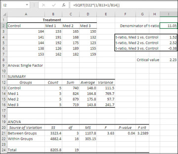
Figure 7.5 When the group sizes are equal, as here, all the comparisons’ t-ratios have the same denominator.
The data is laid out for the Data Analysis tool in A2:D7. The ANOVA: Single Factor tool in the Data Analysis add-in returns the results shown in the range A11:G24. You’ll need the group means, the Mean Square Error from the ANOVA table, and the group counts.
The first step is to calculate the denominator of the t-ratios. With equal group sizes, the same denominator is used for each t-ratio. The formula for the denominator is:

where MSE is the mean square error from the ANOVA table, shown in Figure 7.5 in cell D22. (Mean square error is simply another term for mean square within or mean square residual.)
When, as here, the group sizes are equal, you can also use this arithmetically equivalent formula:

The denominator for the t-ratios in this example is given in cell I2. It uses this formula:
=SQRT(D22*(1/B13+1/B14))
where cell D22 contains the mean square error and cells B13 and B14 contain group counts. With all groups of the same size, it doesn’t matter which group counts you use in the formula. As suggested earlier, with equal group sizes the Excel formula could also be:
=SQRT((2*D22)/B13)
The next step is to find the difference between the mean of each treatment group and the mean of the control group, and divide those differences by the denominator. The result is one or more t-ratios. For example, here’s the formula in cell I4 of Figure 7.5.
=(D14−D13)/I2
The formula divides the difference between the mean of the Med 1 group (D14) and the mean of the Control group (D13) by the denominator of the t-ratio (I2). The formulas in cells I5 and I6 follow that pattern:
I5: =(D15−D13)/I2
I6: =(D16−D13)/I2
At this point you look up the value in the Dunnett tables that corresponds to three criteria:
The Degrees of Freedom Within from the ANOVA table (in Figure 7.5, the value 16 in cell C22)
The total number of groups, including the control group
The value of alpha that you selected before seeing the data from your experiment
Most printed tables give you a choice of 0.05 and 0.01. That’s restrictive, of course, and it delights me that Excel offers exact probabilities for any probability level you might present it for various distributions including the chi-square, the binomial, the t and the F.
For the present data set, the printed Dunnett tables give a critical value of 2.23 for four groups and 16 Degrees of Freedom Within, at the 0.05 alpha level. They give 3.05 at the 0.01 alpha level.
Because the t-ratio in cell I5, which contrasts Med 2 with Control, is the only one to exceed the critical value of 2.23, you could reject the null hypothesis of no difference in the population means for those two groups at the .05 confidence level. You could not reject it at the 0.01 confidence level because the t-ratio does not exceed the 0.01 level of 3.05.
Compare all that with the results shown in Figure 7.6.
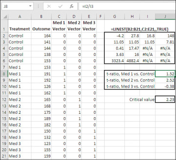
Figure 7.6 Much less calculation is needed when you start by analyzing the data with regression.
Start by noticing that cells G2, H2, and I2, which contain the regression coefficients for Med 3 Vector, Med 2 Vector, and Med 1 Vector (in that order), express the differences between the means of the treatment groups and the control group.
For example, the regression coefficient in cell H2 (27.8) is the difference between the Med 2 mean (175.8, in cell D15 of Figure 7.5) and the Control mean (148.0, in cell D13 of Figure 7.5). So right off the bat you’re relieved of the need to calculate those differences. (You can, however, find the mean of the control group in the regression equation’s constant, in cell J2.)
Now notice the standard errors of the regression coefficients, in cells G3, H3, and I3. They are all equal to 11.05, and in any equal-cell-size situation with dummy coding, the standard errors will all have the same value. That value is also the one calculated from the mean square error and the group sizes in Figure 7.5 (see that figure, cell I2).
So, all you need to do if you start the data analysis with LINEST() is to divide the regression coefficients by their standard errors to get the t-ratios that correspond to the Dunnett procedure. Notice that the t-ratios in cells J8, J9, and J10 are identical to those calculated in Figure 7.5, cells I4, I5, and I6.
Now let’s have a look at a slightly more complicated situation, one in which you have different numbers of subjects in your groups. See Figure 7.7.
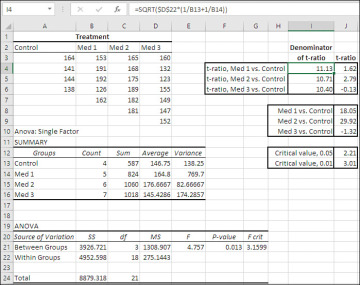
Figure 7.7 Using traditional ANOVA on a data set with unequal group sizes, you need to calculate a different denominator for each t-ratio.
In Figure 7.7, the basic calculations are the same, but instead of using just one denominator as was done in Figure 7.5 (because the groups all had the same number of subjects), we need three denominators because the group sizes are different. The three denominators appear in the range I4:I6, and use the version of the formula given earlier:

So, the formulas to return the t-ratio’s denominator are:
I4: =SQRT($D$22*(1/B13+1/B14))
I5: =SQRT($D$22*(1/B13+1/B15))
I6: =SQRT($D$22*(1/B13+1/B16))
Notice that the only difference between the formulas is that they alter a reference from B14 to B15 to B16, as the number of observations in the Med 1, Med 2, and Med 3 groups increases from 5 to 6 to 7. The formulas make use of the group counts returned by the Data Analysis add-in to pick up the number of observations in each treatment group.
The differences between the treatment group means and the control group mean are shown in the range J8:J10. They are the numerators for the t-ratios, which appear in the range J4:J6. Each t-ratio is the result of dividing the difference between two group means by the associated denominator, as follows:
J4: =J8/I4
J5: =J9/I5
J6: =J10/I6
In sum, when your group sizes are unequal, traditional methods have you calculate different denominators for each of the t-ratios that contrast all group means but one (here, Med 1, Med 2, and Med 3) with another mean (here, Control). Then for each pair of means, calculate the mean difference and divide by the denominator for that pair.
You’ll also want to compare the values of the t-ratios with the values in Dunnett’s tables. In this case you would want to locate the values associated with 18 within-groups degrees of freedom (from cell C22 in the ANOVA table) and 4 groups. The intersection of those values in the table is 2.21 for an alpha level of 0.05 and 3.01 for an alpha level of 0.01 (see cells J12 and J13 in Figure 7.7). Therefore, only the difference between Med 2 and Control, with a t-ratio of 2.79, is beyond the cutoff for 5% of the Dunnett t distribution, and it does not exceed the cutoff for 1% of the distribution. You can reject the null for Med 2 versus Control at the 5% level of confidence but not at the 1% level. You cannot reject the null hypothesis for the other two contrasts at even the 5% level of confidence.
Notice that the F-ratio in the ANOVA table, 4.757 in cell E21, will appear in a central F distribution with 3 and 18 degrees of freedom only 1.3% of the time. (A central F distribution in the context of an ANOVA is one in which the estimate of the population variance due to the differences among group means is equal to the estimate of the population variance due to the average within-group variance.) So the ANOVA informs you that an F-ratio of 4.757 with 3 and 18 degrees of freedom is unlikely to occur by chance if the population means equal one another.
That likelihood, 1.3%, echoes the result of the contrast of the Med 2 group with the Control group. The t-ratio for that contrast, 2.79, exceeds the critical value for 5% of the Dunnett distribution but not the critical value for 1% of the distribution. So the objective of the multiple comparison procedure, to pinpoint the difference in means that the ANOVA’s F-ratio tells you must exist, has been met.
Things go a lot more smoothly if you use LINEST() instead. See Figure 7.8.
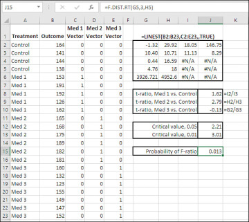
Figure 7.8 LINEST() calculates the mean differences and t-ratio denominators for you.
Figure 7.8 has the same underlying data as Figure 7.7: Four groups with a different number of subjects in each. (The group membership vectors were created just as shown in Figure 7.6, using VLOOKUP(), but to save space in the figure the formulas were converted to values and the key deleted.)
This LINEST() formula is array-entered in the range G2:J6:
=LINEST(B2:B23,C2:E23,,TRUE)
Compare the regression coefficients in cells G2, H2, and I2 with the mean differences shown in Figure 7.7 (J8:J10). Once again, just as in Figures 7.5 and 7.6, the regression coefficients are exactly equal to the mean differences between the groups that have 1’s in the vectors and the group that has 0’s throughout. So there’s no need to calculate the mean differences explicitly.
The standard errors of the regression coefficients in Figure 7.8 also equal the denominators of the t-ratios in Figure 7.7 (in the range I4:I6). LINEST() automatically takes the differences in the group sizes into account. All there’s left to do is divide the regression coefficients by their standards errors, as is done in the range J8:J10. The formulas in those cells are given as text in K8:K10. But don’t forget, when you label each t-ratio with verbiage that states which two means are involved, that LINEST() returns the coefficients and their standard errors backwards: Med 3 versus Control in G2:G3, Med 2 versus Control in cell H2:H3, and Med 1 versus Control in I2:I3.
Figure 7.8 repeats in J12 and J13 the critical Dunnett values for 18 within-group degrees of freedom (picked up from cell H5 in the LINEST() results) and 4 groups at the 0.05 and 0.01 cutoffs. The outcome is, of course, the same: Your choice of whether to use regression or traditional ANOVA makes no difference to the outcome of the multiple comparison procedure.
Finally, as mentioned earlier, the LINEST() function does not return the probability of the F-ratio associated with the R2 for the full regression. That figure is returned in cell J15 by this formula:
=F.DIST.RT(G5,3,H5)
Where G5 contains the F-ratio and H5 contains the within-group (or “residual”) degrees of freedom. You have to supply the second argument (here, 3) yourself: It’s the number of groups minus 1 (notice that it equals the number of vectors in LINEST()’s second argument, C2:E23) also known as the degrees of freedom between in an ANOVA or degrees of freedom regression in the context of LINEST().